threejs-procedural-materials skill (Threejs-Awesome-Graphics-Agent-Skills)
- Install
- SKILL.md (verbatim)
- Material graph order
- Required controls
- Failure conditions
- Routing boundary
- Other files in this skill
- assets/raytraced-diamond/THIRDPARTYLICENSES.md (verbatim)
- references/dielectric-glass-optics.md (verbatim)
- Contents
- Two-pass ownership
- Back-face data buffer
- Interior exit search
- Interface response and the bounce budget
- Volume absorption from a tint
- Spectral path and dispersion
- Environment probe and the visible surround
- Choosing between geometric and image-space transmission
- Limits and failure patterns
- Diagnostics
- references/hybrid-soil-moss-surface.md (verbatim)
- Contents
- Hybrid implementation boundary
- Shared height ownership
- Soil identity fields
- Ground moss identity and height
- Model moss accumulation
- PBR channel coupling
- Diagnostics
- Default parameter contract
- Mound formula
- Crack formula
- Texture contract
- Failure modes
- references/physical-diffraction-grating.md (verbatim)
- Contents
- Surface and layer contract
- Embossed microstructure fields
- Spectral reconstruction
- Phase-grating response
- Strip-emitter integration
- Stable object-space frame
- Observed limits and defects
- Diagnostics
- references/procedural-pbr-system.md (verbatim)
- Contents
- Atlas block material
- Atlas and minification response
- Shared shadow/light causes
- Planetary node material
- Game terrain and pooled debris
- Gallery authored PBR identities
- Selection rules and limitations
- Diagnostics
What it does. Author production procedural materials in Three.js. Use for hybrid texture-backed PBR soil and moss with procedural displacement and masks, upward-facing model moss accumulation, atlas filtering, specular AA, planet-space fields, terrain wetness, lava and emissive surfaces, reflective wave-optical diffraction gratings, air-film-air soap bubbles with Airy interference, raytraced diamond and gem refraction with internal reflection and dispersion, image-space glass transmission with spectral dispersion and volume absorption, deforming softbody jelly materials with XPBD mechanics and refractive caustics, per-instance dissolve, authored PBR identities, derivative normals, and custom direct-light shadow modulation. Part of scottstts/Threejs-Awesome-Graphics-Agent-Skills (scottstts/Threejs-Awesome-Graphics-Agent-Skills).
| Upstream | scottstts/Threejs-Awesome-Graphics-Agent-Skills |
| Skill file | skills/threejs-procedural-materials/SKILL.md |
| License | MIT |
| Author | Scott Sun (scottstts) |
| Fetched | 2026-09-10 |
Install
npx skills add scottstts/Threejs-Awesome-Graphics-Agent-Skills --skill threejs-procedural-materials, or copy the skill folder into~/.claude/skills/threejs-procedural-materials/.- Raw file:
curl -sL https://raw.githubusercontent.com/scottstts/Threejs-Awesome-Graphics-Agent-Skills/HEAD/skills/threejs-procedural-materials/SKILL.md
SKILL.md (verbatim)
name: threejs-procedural-materials
description: Author production procedural materials in Three.js. Use for hybrid texture-backed PBR soil and moss with procedural displacement and masks, upward-facing model moss accumulation, atlas filtering, specular AA, planet-space fields, terrain wetness, lava and emissive surfaces, reflective wave-optical diffraction gratings, air-film-air soap bubbles with Airy interference, raytraced diamond and gem refraction with internal reflection and dispersion, image-space glass transmission with spectral dispersion and volume absorption, deforming softbody jelly materials with XPBD mechanics and refractive caustics, per-instance dissolve, authored PBR identities, derivative normals, and custom direct-light shadow modulation.
Procedural Materials
Build a material from surface identity and causes. Color, roughness, metalness, normal, transmission, and emission should describe the same surface—not unrelated noise textures.
This skill contains exemplary examples and assets beyond descriptive guidance, they're worth studying, referencing, or even copying. Use them sufficiently when relevant and do NOT blindly skip them.
Material graph order
stable coordinates
  → structural fields
  → material identity weights
  → causal modifiers
  → filtered microstructure
  → PBR channels
  → lighting/shadow extensions
Read references/procedural-pbr-system.md for atlas filtering, specular AA, planetary coordinates, world-height wetness, per-instance dissolve, and authored PBR response bundles.
Read the sculpted gallery frame geometry for walnut, antique-gold, and ebony texture/roughness/metalness/clearcoat bundles under a grazing-light setup.
Read the procedural planet surface for shared geological, climate, water, biome, roughness, and derivative-normal causes on a procedural planetary surface.
Read the analytic wave optics for coupled reflection, refraction, absorption, filtered microstructure, resolved crest response, and their diagnostic channels.
Read the lava flow surface material for raymarched procedural height fields whose normals, rock/lava identity, emission, glow, embers, fog, and grain are coupled to one material cause stack.
Read the raytraced diamond material for a gem whose mesh is its own optical volume: camera-ray entry refraction, a GPU BVH first-hit loop with bounded total-internal-reflection bounces, per-channel IOR dispersion, mip-correct environment exit sampling, and live camera-matrix uniforms.
Read the spectral dispersive glass material for a transmissive body solved in image space: a double-sided back-face data pass with inverted depth, an iterative interior exit search, bounded total internal reflection, Beer-Lambert absorption over the true path length, and a per-wavelength Cauchy index recombined through CIE 1931. Its reusable optical primitives — exact unpolarised Fresnel, Cauchy coefficients, spectral weights, the rotatable environment probe, and the buffer projection — live in glass optics, and references/dielectric-glass-optics.md carries the two-pass contract, buffer format, search bounds, and transmission diagnostics.
Pick between the two transmissive paths by geometry, not by quality. A closed faceted gem whose exit facet must be exact even when it faces away from the camera takes the BVH path. A scanned, assembled, open-sheet, or multi-shell body takes the image-space path, which tolerates inconsistent winding and authored normals pointing either way but cannot see a surface outside the frame.
Read references/physical-diffraction-grating.md for the exact embossed-field, CIE/blackbody spectral, phase-grating, Bessel order-efficiency, coherence-broadening, strip-emitter, additive-layer, stable object-frame, limitation, and diagnostic contracts.
Read the
physical diffraction-grating implementation
for a printed substrate plus additive HDR foil response whose star and stripe
masks select local groove angle, pitch, and relief while wavelength alone owns
spectral colour. Its complete optical model is expressed as a pure TSL graph
with Fn, If, and Loop, without embedded native shader source.
Read references/thin-film-soap-bubble-system.md for the air-film-air Airy equation, representative RGB spectral bands, two-membrane blending, bounded secondary reflection, capillary mechanics, camera-aware inflow, puncture retraction, limits, and diagnostics.
Read the thin-film soap bubble system when soap-film interference must drive the image: it provides wavelength- dependent aqueous index, front and rear membrane passes, analytic nearby- bubble reflection, volume-preserving capillary modes, buoyancy and drag, Taylor-Culick rupture, visible-drop aftermath, and deterministic physics gates.
Read the softbody jelly implementation for a deforming flower-shaped transmissive body whose tetrahedral XPBD state, smooth optical shell, view-ray thickness, BVH refraction, absorption, receiver shadow, and finite RGB caustic fields remain coupled.
Read references/softbody-jelly.md for the softbody coordinate contract, neo-Hookean XPBD split, damping and sleep rules, refractive receiver budget, material constants, limits, and diagnostics.
Required controls
- real or perceptual texture scale;
- material identity weights;
- roughness range and micro-normal strength;
- the causal fields required by the selected material pattern;
- for a transmissive body, the physical constants that define it — index and Abbe pair, interior path budget, extinction depth — named rather than buried inside expressions;
- for a soap film, the exterior and film indices, nanometre thickness range, wavelength bands, surface tension, and membrane ordering;
- distance/derivative filtering;
- specular antialiasing;
- channel and mask debug modes.
- emissive-material debug modes when the material owns glow or volumetric accumulation.
Read references/hybrid-soil-moss-surface.md and the hybrid soil and moss implementation for texture-backed soil and moss albedo, AO, roughness, and normal microdetail combined with procedural mound displacement, moisture, moss coverage/height, and warped cellular cracks. Do not describe its surface identity as fully procedurally synthesized. When moss must also settle onto a model, read the model moss implementation for model-locked coverage, upward-face accumulation, displaced thickness, and shared moss PBR identity.
Failure conditions
- every PBR channel samples independent noise;
- roughness is a scalar afterthought;
- high-frequency normals survive below one pixel;
- triplanar projection has visible orientation or scale seams;
- atlas padding is ignored under mipmapping;
- custom lighting removes energy conservation without an explicit stylized goal;
- post-processing is used to hide unstable highlights.
- diffraction hue is painted from UV instead of derived from wavelength;
- a groove frame follows the camera or world axes instead of the object;
- a narrowed diffraction lobe loses energy because its density lacks sigma normalization.
- a soap bubble is treated as a solid glass sphere or painted with a rainbow instead of using air-film-air interference;
- a deformed soap membrane retains the undeformed sphere normal;
- a deforming transmissive body updates its render shell, optical BVH, and receiver field from different states;
- a finite caustic receiver lets non-zero data reach its clamped texture edge;
- a softbody solver uses variable integration steps or an uncoupled rest-stress split that injects energy after damping;
Routing boundary
Use $threejs-procedural-fields when the main problem is designing shared
scalar/vector causes. Use $threejs-procedural-planets for a complete
orbit-to-close-approach body, not merely its material. Use
$threejs-parallax-occlusion-mapping when a height field must own ray-marched
intersection, silhouette coverage, or relief-aware shadows. Use
$threejs-temporal-surfaces for view-aligned wet-glass optics and screen-space
history; this skill owns the optical path through a transmissive body itself.
Other files in this skill
- agents/openai.yaml
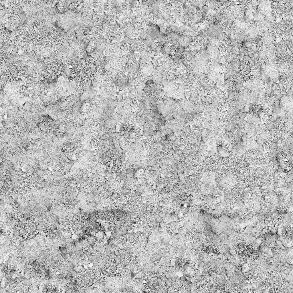
- assets/hybrid-soil-moss-surface/Ground103_1K-JPG_AmbientOcclusion.jpg
- assets/hybrid-soil-moss-surface/Ground103_1K-JPG_Color.jpg
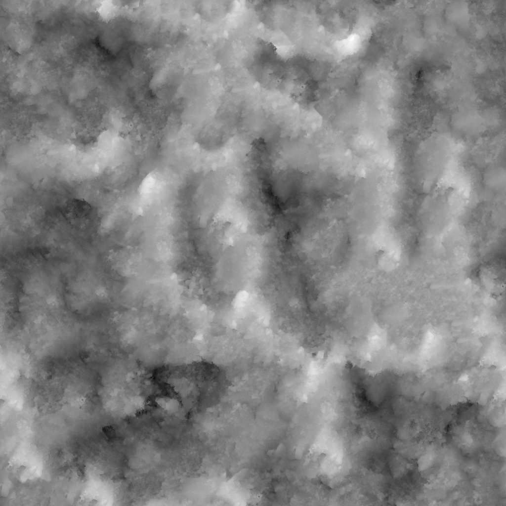
- assets/hybrid-soil-moss-surface/Ground103_1K-JPG_Displacement.jpg
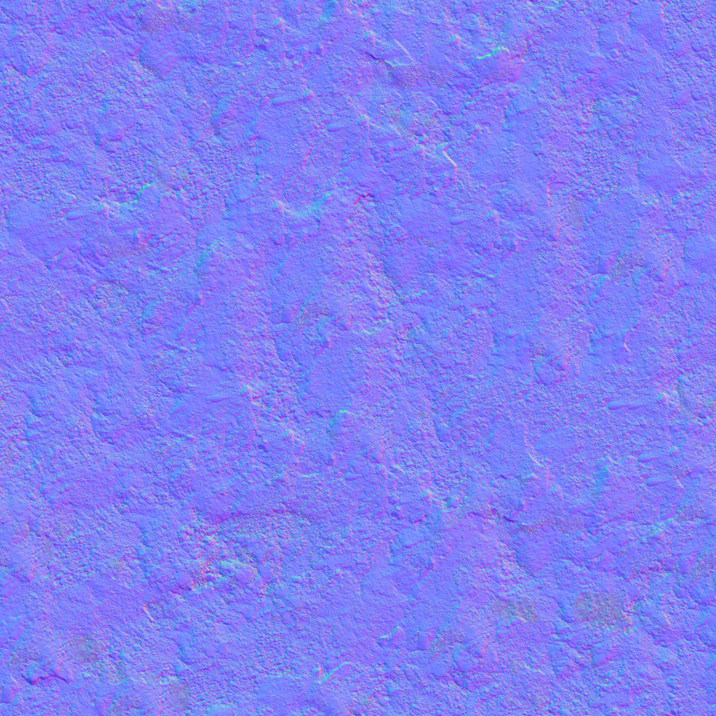
- assets/hybrid-soil-moss-surface/Ground103_1K-JPG_NormalGL.jpg
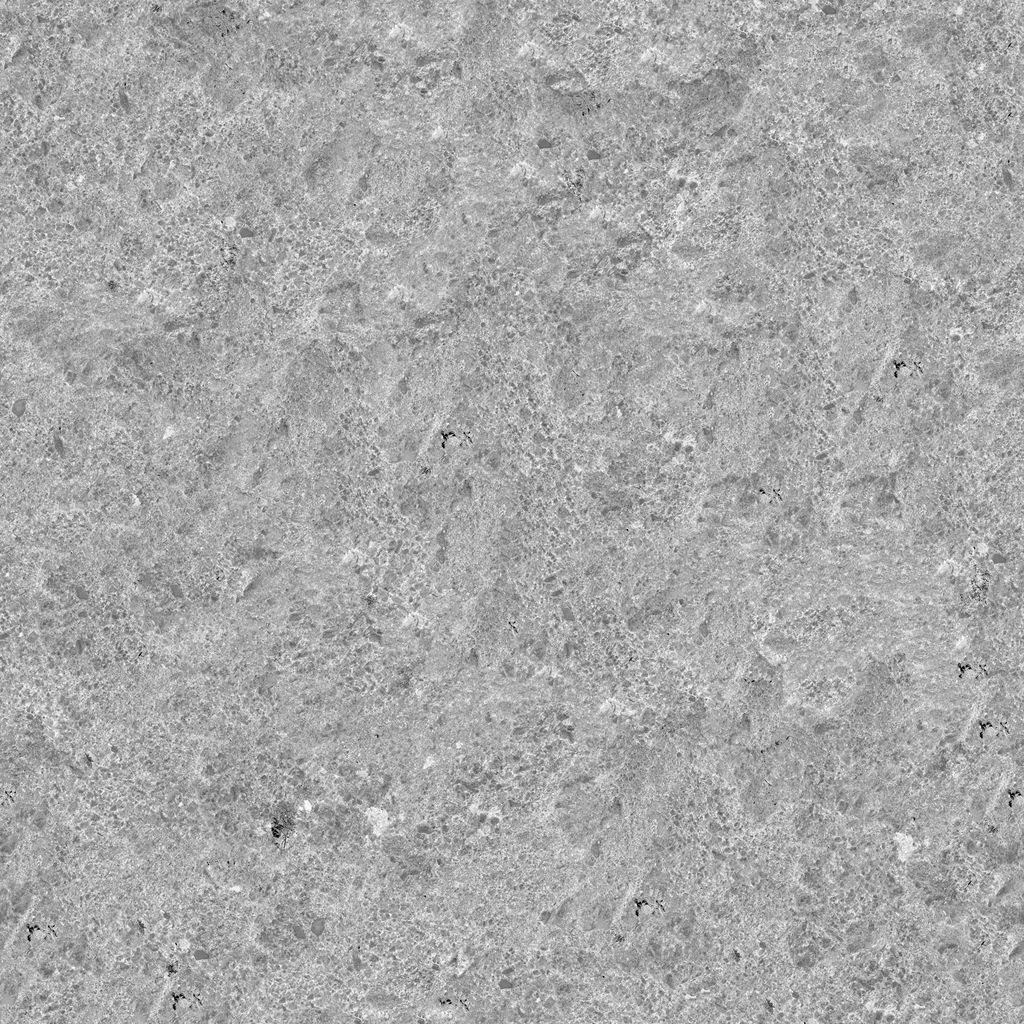
- assets/hybrid-soil-moss-surface/Ground103_1K-JPG_Roughness.jpg
- assets/hybrid-soil-moss-surface/moss/Moss002_1K-JPG_AmbientOcclusion.jpg
- assets/hybrid-soil-moss-surface/moss/Moss002_1K-JPG_Color.jpg
- assets/hybrid-soil-moss-surface/moss/Moss002_1K-JPG_NormalGL.jpg
- assets/hybrid-soil-moss-surface/moss/Moss002_1K-JPG_Roughness.jpg
- assets/raytraced-diamond/THIRD_PARTY_LICENSES.md
- assets/raytraced-diamond/diamond.glb
- examples/hybrid-soil-moss-surface/hybrid-soil-moss-surface.js
- examples/hybrid-soil-moss-surface/model-moss-accumulation.js
- examples/lava-flow-surface/lava-surface.js
- examples/physical-diffraction-grating/physical-diffraction-grating.js
- examples/raytraced-diamond/diamond-material.js
- examples/softbody-jelly/softbody-jelly.js
- examples/spectral-dispersive-glass/glass-optics.js
- examples/spectral-dispersive-glass/spectral-glass-material.js
- examples/thin-film-soap-bubbles/soap-bubble-system.js
- references/dielectric-glass-optics.md
- references/hybrid-soil-moss-surface.md
- references/physical-diffraction-grating.md
- references/procedural-pbr-system.md
- references/softbody-jelly.md
- references/thin-film-soap-bubble-system.md


assets/raytraced-diamond/THIRD_PARTY_LICENSES.md (verbatim)
Third-party asset notices
The faceted diamond model diamond.glb in this directory is a third-party
asset used under the MIT License reproduced below.
MIT License
Copyright (c) 2022 N8python
Permission is hereby granted, free of charge, to any person obtaining a copy of this software and associated documentation files (the "Software"), to deal in the Software without restriction, including without limitation the rights to use, copy, modify, merge, publish, distribute, sublicense, and/or sell copies of the Software, and to permit persons to whom the Software is furnished to do so, subject to the following conditions:
The above copyright notice and this permission notice shall be included in all copies or substantial portions of the Software.
THE SOFTWARE IS PROVIDED "AS IS", WITHOUT WARRANTY OF ANY KIND, EXPRESS OR IMPLIED, INCLUDING BUT NOT LIMITED TO THE WARRANTIES OF MERCHANTABILITY, FITNESS FOR A PARTICULAR PURPOSE AND NONINFRINGEMENT. IN NO EVENT SHALL THE AUTHORS OR COPYRIGHT HOLDERS BE LIABLE FOR ANY CLAIM, DAMAGES OR OTHER LIABILITY, WHETHER IN AN ACTION OF CONTRACT, TORT OR OTHERWISE, ARISING FROM, OUT OF OR IN CONNECTION WITH THE SOFTWARE OR THE USE OR OTHER DEALINGS IN THE SOFTWARE.
references/dielectric-glass-optics.md (verbatim)
Dielectric glass optics
Use this reference when a body has to transmit its surroundings rather than merely look shiny: cast and blown glass, crystal, resin, ice blocks, gemstone substitutes, and any material whose interior path — not its surface — produces the image.
A transmissive body is not a PBR channel bundle with the opacity turned down. It is a path: enter, travel, hit the far interface, either leave or bounce, and carry a wavelength-dependent index and a per-unit-length extinction the whole way. Every mechanism below exists to keep one of those stages honest.
Contents
- Two-pass ownership
- Back-face data buffer
- Interior exit search
- Interface response and the bounce budget
- Volume absorption from a tint
- Spectral path and dispersion
- Environment probe and the visible surround
- Choosing between geometric and image-space transmission
- Limits and failure patterns
- Diagnostics
Two-pass ownership
The material owns two passes and the buffer between them:
pass 1  subject meshes → back-face data target (world normal, camera distance)
pass 2  camera pass: glass material reads that target per fragment
Ordering is a contract, not an optimisation. Pass 1 runs every frame, before the camera pass, with the same camera. A buffer left over from the previous frame refracts the previous frame's silhouette, which reads as a body whose interior lags the camera by one frame — most visible while orbiting.
The target tracks the drawing-buffer size in physical pixels, because the interior ray addresses it by projecting world points into that exact space.
Back-face data buffer
The spectral-dispersive-glass example allocates:
format          RGBA, HalfFloatType
filtering       NearestFilter (min and mag)
mipmaps         disabled
depth buffer    enabled
contents        xyz = geometric world normal, w = distance to camera
Three properties of the pass matter more than the format:
- Double-sided, no culling. A body assembled from several interpenetrating shells has no consistent winding, so a facing test picks the wrong triangles. Rasterise everything.
- Inverted fragment depth. Writing
1 − depthmakes the default less-than test keep the farthest surface along each view ray. That surface is the exit of the union hull, which is the interface refraction should target. Without the inversion, the buffer holds the nearest back face and interiors collapse to a thin skin. - A pure geometric normal. Store
normalize(modelNormalMatrix * normalLocal)— never a normal already flipped toward the viewer by the rasteriser. The consuming pass re-orients the stored vector along the ray it is currently following, so authored normal direction stops mattering.
Half float is required, not preferred: w is a scene-scale distance and the
normal is signed. Nearest filtering is also required — linear filtering across
a silhouette blends two unrelated surfaces into a distance that lies between
them, and the exit search then lands in empty space.
Interior exit search
The exit point is found by projection and refinement rather than by
intersection. Per segment, EXIT_REFINEMENTS = 3 passes of:
Pest = orig + dir * tSeg                    estimated exit point
uv   = clamp(projectToBufferUV(Pest), 0, 1) where the camera sees that point
bb   = backFaceData(uv)                     surface stored under that texel
Pb   = camP + normalize(Pest − camP) * bb.w rebuilt world position
tSeg = clamp(dot(Pb − orig, dir), minWall, maxSegment)
The rebuild matters. The buffer stores a distance along the camera ray through
that texel, not along the interior ray, so the surface point has to be
reconstructed before the segment length is measured along dir.
The seed for the first segment is the view-ray thickness at the fragment:
bb.w − distFront, floored at the minimum wall. Where the buffer holds nothing
— the silhouette rim, where the exit surface projects outside the visible
buffer — the seed falls back to 0.015 × bounding diagonal.
Bounds, both derived from the subject's world bounding-box diagonal:
MIN_WALL = 0.08world units at the example's normalised subject scale. Open, zero-volume sheets would otherwise transmit over no path length at all and lose their tint completely.MAX_SEGMENT_RATIO = 3.0 × diagonal. A refinement that lands on an unrelated distant surface would otherwise stretch one segment across the whole scene.
Three passes converge on gently curved bodies. They cannot recover a surface the camera never saw; that is the standing cost of solving this in image space.
Interface response and the bounce budget
Every interface uses exact unpolarised Fresnel reflectance:
sin²θt = (n1/n2)² (1 − cos²θi)
cosθt  = sqrt(max(1 − sin²θt, 1e-6))
r_s    = (n1 cosθi − n2 cosθt) / (n1 cosθi + n2 cosθt)
r_p    = (n2 cosθi − n1 cosθt) / (n2 cosθi + n1 cosθt)
F      = sin²θt ≥ 1 ? 1 : clamp(0.5 (r_s² + r_p²), 0, 1)
Schlick is not interchangeable here. The interior path spends most of its interfaces near grazing incidence, exactly where the approximation drifts, and it never reaches 1 at the critical angle — so total internal reflection leaks energy out of the body instead of trapping it.
Returning 1 past the critical angle is what makes TIR fall out of the same
expression. The segment loop needs no separate test: it refracts out with
weight 1 − F, multiplies the running throughput by F, reflects, and
continues.
Budget in the example: PATH_SEGMENTS = 4 (TIR bounces plus the exit that
ends the path), with an early Break once throughput drops below
THROUGHPUT_CUTOFF = 0.004. After the last segment, the remaining throughput
leaves along the current direction and is added as residual energy. Omitting that
residual term darkens the deepest parts of the body, where paths are most
likely to exhaust the budget.
Entry incidence is clamped to [1e-4, 1] and exit incidence likewise, so
grazing fragments cannot divide by zero at the silhouette.
Volume absorption from a tint
Transmission is attenuated by Beer-Lambert over the accumulated internal path length, not by a flat colour multiply:
σ      = −ln(clamp(t, 1e-4, 1)) / max(depth, 1e-3)   [1/unit]
L_out  = L_in · exp(−σ · s)                          s = path length so far
Inverting the exponential keeps the control perceptual — choose the colour a chosen thickness should show — and, more importantly, keeps one body internally consistent: thin edges and thick cores read the same σ over their own path lengths, which is what makes cast glass look solid rather than surface-tinted.
The spectral-dispersive-glass example uses tint = #d0edda at depth = 0.5
world units, which resolves to σ ≈ (0.922, 0.332, 0.710) 1/unit.
Decode the tint exactly once, and decode it explicitly. A Color built from an
sRGB literal is already in the linear working space, so an added
convertSRGBToLinear() squares the transfer and inflates extinction by roughly
2.3×. Nothing about the image announces this: doubling only deepens the tint,
so tuning by eye absorbs the error while the picker quietly stops meaning what
it says, and the mistake then travels with the tuned literal. It also drifts
with saturation rather than scaling uniformly — a mid-grey tint moves from
σ 3.07 to 6.53 1/unit — so the depth control becomes least predictable
exactly where the tint is strongest. Parse the literal as
LinearSRGBColorSpace to keep its raw components and apply the one decode
yourself; σ is then identical whether or not colour management is enabled.
Spectral path and dispersion
Dispersion is a property of the index, so it belongs ahead of the whole path,
not in a post-hoc channel offset. The index comes from the two numbers
glass catalogues publish, n_d and the Abbe number V_d:
K = 1/486.13² − 1/656.27²      nm⁻²   (F and C Fraunhofer lines)
B = (n_d − 1) / (V_d · K)      nm²
A = n_d − B / 589.29²
n(λ) = A + B / λ²
A and B are constant for a given glass and resolve on the CPU; only
A + B/λ² belongs in the shader. The example ships n_d = 1.5, V_d = 32 —
crown-glass index with flint-like fire.
The whole interior path is then traced once per wavelength sample.
SPECTRAL_SAMPLES = 8 stratified centres span 415–695 nm, deliberately
narrower than the full visible range because the colour matching curves are
near zero at both ends. Each sample is weighted by CIE 1931 colour matching,
built from multi-lobe piecewise Gaussians and converted XYZ → linear sRGB:
X = 1.056 g(λ;599.8,37.9,31.0) + 0.362 g(λ;442.0,16.0,26.7) − 0.065 g(λ;501.1,20.4,26.2)
Y = 0.821 g(λ;568.8,46.9,40.5) + 0.286 g(λ;530.9,16.3,31.1)
Z = 1.217 g(λ;437.0,11.8,36.0) + 0.681 g(λ;459.0,26.0,13.8)

g(λ; μ, s₁, s₂) = exp(−½ t²),  t = (λ − μ) / (λ < μ ? s₁ : s₂)
Accumulate weight · radiance and weight separately and divide at the end,
guarding the divisor at 1e-4. That running normalisation is what guarantees a
dispersion-free spectrum reconstructs the environment exactly instead of
picking up a cast, and it keeps the image stable when the sample count changes.
Individual weights are legitimately negative outside the sRGB gamut, so clamp
the final sum — never the per-sample weights.
Below roughly six samples the fire separates into discrete coloured copies of the environment rather than a continuous spread. Cost scales linearly: each sample re-traces every segment.
Environment probe and the visible surround
Both the external specular reflection and every exit ray read one equirectangular HDR probe, sampled at an explicit mip level. Explicit is mandatory, not stylistic: every lookup on the interior path sits inside a non-uniform loop, where implicit derivatives are undefined.
Probe requirements:
mapping      EquirectangularReflectionMapping
wrapS        RepeatWrapping        closes the horizontal seam
wrapT        ClampToEdgeWrapping   keeps the poles from wrapping together
mipmaps      enabled               explicit LOD needs a chain to walk
filtering    LinearMipmapLinear / Linear
The mip level doubles as surface micro-roughness: level 0 is polished glass, higher levels integrate a wider cone of incoming radiance and read as frost. The example ships level 0 and a probe rotation of 0 rad.
Assign the same probe as the scene background. What the viewer sees through the body has to be the radiance field they see around it, or the body reads as a cutout of an unrelated scene — a mismatch that no amount of index tuning fixes.
Derive the background direction from the geometric world normal, never from
positionWorld − cameraPosition. A background node is drawn on a unit sphere
the renderer owns, and nothing in the contract says where that sphere sits;
renderers have both centred it on the camera and left it at the world origin.
Where it sits at the origin, a position-derived direction compresses the whole
view into a cone of half-angle asin(1 / |cameraPosition|) around the
camera-to-origin axis. At a camera distance of 2.86 units that is a 41° cone
covering the full screen. The failure is quiet: the background still looks like
a plausibly lit environment, just magnified and warped, which reads as a
low-resolution probe rather than a wrong direction. A sphere's outward normal
is translation invariant and stays correct under either placement.
The material returns unbounded linear radiance. The host owns exposure and the display transform, which must handle values well above 1; a clamped transform crushes exactly the caustic-like concentrations this path exists to produce.
Choosing between geometric and image-space transmission
Two transmission strategies belong to different geometry, not different quality tiers:
| image-space path | geometric path | |
|---|---|---|
| exit surface from | back-face data buffer | BVH first hit against the mesh |
| tolerates open sheets, multiple shells, bad winding | yes | no |
| sees surfaces outside the frustum or occluded | no | yes |
| dispersion model | per-wavelength Cauchy index | per-channel index offset |
| cost driver | samples × segments × buffer reads | bounces × BVH traversal |
Use the spectral-dispersive-glass example for scanned, assembled, or
non-watertight bodies, and where dispersion has to track a real catalogue
index. Use the raytraced-diamond example for closed faceted gems, where the
cut itself produces the optical result and the exit facet must be exact even
when it faces away from the camera.
Limits and failure patterns
- Off-screen exits are unknowable. Any interior ray whose exit projects outside the buffer falls back to the assumed wall thickness. Wide-angle framing and bodies that overflow the frame expand this region.
- Occluded exits resolve to the occluder. The buffer holds one surface per texel; if another object is in front, the search reads that object's distance. Render only the transmissive subject into the data pass.
- A moving subject must be followed into the data pass. The pass draws its
own copy of the hierarchy, so every pose change has to reach that copy before
it renders, or the visible surface moves while the stored back faces do not
and the interior refracts a pose the body no longer holds. The
spectral-dispersive-glassexample follows the root's world transform — so ancestor motion counts — plus each descendant's local matrix, visibility, and morph weights, every pass. Geometry buffers and skeletons are shared by reference, so vertex edits and skinned animation need nothing. Structural change is the exception: meshes added or removed, or a geometry swapped, need the copy rebuilt, because the node pairing is fixed when it is built. - No caustics, no shadow transport. This path resolves what the body shows, not what it casts. Light it as an unshadowed transmissive object.
- A dense subject pays twice. The data pass rasterises the full triangle count double-sided every frame, in addition to the camera pass.
- Cost is multiplicative. Samples × segments × three refinements × two buffer reads per refinement is the per-fragment budget; halving the sample count is the cheapest lever, followed by the segment budget.
- A flipped V still looks plausible. The projection inverts V for backends that rasterise render targets with Y flipped relative to the classic GL convention. A wrong choice produces a coherent but incorrect interior.
Diagnostics
The material can output three channels in place of the final image. Read them in this order — each one clears a stage before the next becomes meaningful.
| view | shows | failure it exposes |
|---|---|---|
| view-ray thickness | (bb.w − distFront) / (0.6 × diagonal) |
black interior means the data pass wrote nothing; a flat mid-grey body means the depth inversion is missing and only the near skin is stored |
| back-face normal | stored normal, ×0.5 + 0.5 |
noise or single-colour fields mean winding or the normal matrix is wrong; black regions mark texels with no data, which is exactly where the fallback thickness applies |
| entry Fresnel | F(cosθi, 1 → n_d) |
the only term independent of the interior path. If this looks right and the final image does not, the defect is in the exit search, not the surface response |
Further checks that are worth running once per integration:
- Ground-truth the projection. Compare the buffer against a CPU raycast mask of the same frame before trusting any interior result.
- Collapse the spectrum. One sample at
λ_dmust reconstruct the environment with no colour cast. A cast means the weight normalisation is broken. - Zero the absorption. With
σ = 0, total radiance must not exceed the probe's brightest value; excess means throughput is being double-counted across segments. - Single segment. With one segment the body must show refraction but no internal structure. Structure at one segment means the residual term is being added inside the loop rather than after it.
references/hybrid-soil-moss-surface.md (verbatim)
Hybrid PBR soil and moss surface
Contents
- Hybrid implementation boundary
- Shared height ownership
- Soil identity fields
- Ground moss identity and height
- Model moss accumulation
- PBR channel coupling
- Diagnostics
- Default parameter contract
- Mound formula
- Crack formula
- Texture contract
- Failure modes
Hybrid implementation boundary
Treat this example as a hybrid texture-backed and procedural material. The soil and moss texture sets provide albedo, AO, roughness, and tangent-space normal microdetail. Procedural fields provide mound displacement, macro normals, tone and moisture variation, cracks, moss coverage and thickness, and model accumulation. The displacement texture is loaded with the PBR set but disabled; procedural height owns the silhouette.
Do not call the soil or moss appearance fully procedural and do not imply that their PBR texture channels are synthesized by the shader.
Shared height ownership
Use one world-XZ field for broad mound displacement and finite-difference relief normals. The field combines five-octave simplex fBm, a coverage threshold, finer drift, and a rim taper. Read the hybrid soil and moss implementation for the exact uniforms, shader injection points, and defaults.
Soil identity fields
Keep three independently positioned but causally meaningful masks:
- broad tone variation multiplies the base albedo;
- moisture darkens albedo and lowers roughness together;
- warped two-scale Worley borders create recessed dry cracks.
The crack field must drive color, roughness, and groove normals. The moisture field must drive color and roughness. Do not replace either with unrelated channel noise.
Ground moss identity and height
Use one world-XZ fBm mask for both moss coverage and raised moss thickness.
Add mossHeightAt to groundHeightAt, then reuse the same coverage for moss
albedo, AO, roughness, and normal-map blending. Read
the hybrid soil and moss implementation
for the exact mask, rim taper, shader stages, texture loading, and defaults.
Keep the moss baseline together:
enabled             0 by default
patch scale         0.14
coverage            0.55
patch edge          0.14
thickness           0.14 world units
relief scale        0.90
relief strength     0.70
texture scale       0.35 tiles per world unit
roughness           1.00
normal strength     1.00
AO strength         1.00
Model moss accumulation
Read the model moss implementation when moss must settle on an arbitrary GLB. Share the ground moss maps, tint, and master enable uniform by reference. Compute coverage in model-locked XZ coordinates, gate it by the world-normal upward component, and displace along the local normal after converting the desired world thickness through the mesh scale. Refresh the group world-to-model matrix after transforms.
Keep these model defaults together:
coverage            0.70
patch scale         0.90
patch edge          0.15
thickness           0.05 world units
upward threshold    0.35
texture scale       2.00
roughness           1.00
AO strength         1.00
relief strength     0.50
relief scale        3.00
PBR channel coupling
Use the included soil and moss albedo, AO, roughness, and OpenGL normal maps as the texture-backed PBR identity. Tile each material's channels consistently. Keep texture displacement disabled because procedural mound and moss height own the silhouette; use texture normals for microstructure and finite- difference procedural fields for macro relief.
Diagnostics
Expose final, mound height, moisture, crack, and moss masks. Permit a ground-only view when a model is present. Report seed, mound coverage, moss coverage, moisture coverage, crack enablement, and texture scale.
Default parameter contract
Keep this visual baseline together:
mound scale       0.12
mound depth       0.55 world units
mound coverage    1.00
mound edge        0.15
fine relief scale 0.70
fine strength     0.60
tone scale        0.08
tone amount       0.28
moisture scale    0.18
wet darkening     0.50
wet roughness     0.35
crack amount      0.75
crack scale       0.90
crack width       0.06
crack depth       0.70
macro normal mix  0.70
Treat scales as world-XZ frequencies. Seeds are two-dimensional field offsets, not random numbers sampled per frame.
Mound formula
float base = fbm(worldXZ * uMoundScale + uSeed) * 0.5 + 0.5;
float drift = fbm(worldXZ * uBumpScale + uSeed * 0.5) * 0.5 + 0.5;
float h = base * (1.0 - 0.4 * uBumpStrength
                        + 0.4 * uBumpStrength * drift);
float threshold = mix(1.0 + uMoundEdge,
                      -uMoundEdge,
                      uMoundCoverage);
h *= smoothstep(threshold - uMoundEdge,
                threshold + uMoundEdge,
                base);
Taper the field over the final two world units of a plane with half-extent ten. If the host has a different extent, parameterize the taper rather than silently stretching this constant.
Crack formula
Evaluate Worley F1/F2 border distance twice. The secondary field runs at 2.7
times the primary coordinate and contributes half strength. Form the final
channel with max(primary, secondary). Apply optional fBm warp before both
evaluations so the large and small fissures remain related.
primary   = 1 - smoothstep(0, width, F2 - F1)
secondary = (1 - smoothstep(0, width * 1.6, F2b - F1b)) * 0.5
crack     = saturate(max(primary, secondary)) * amount
Texture contract
Decode only the color map as sRGB. Keep AO, roughness, OpenGL tangent normal,
and displacement maps linear. Use repeat wrapping, identical repeat values,
and the renderer's supported anisotropy. Supply uv1 for AO on current Three.js
versions. Keep metalness at zero and base roughness at one before maps and
procedural modifiers.
Failure modes
- texture normal and procedural macro normal use incompatible spaces;
- wet soil darkens but remains equally rough;
- cracks are an albedo decal without groove response;
- geometry uses a different mound field from shading;
- changing coverage changes the seed or spatial frequency;
- the plane edge ends in an unsupported vertical cliff;
- ground moss color and raised height use different masks;
- model moss swims because coverage is evaluated in world coordinates;
- model scale changes the apparent world-space moss thickness;
- ground and model moss use unrelated PBR texture identities.
references/physical-diffraction-grating.md (verbatim)
Physical diffraction grating
Use this reference for reflective embossed foil whose colour is produced by a wave-optical grating under a real emitter direction, rather than by a rainbow texture, a time-driven UV band, or framebuffer colour separation.
Contents
- Surface and layer contract
- Embossed microstructure fields
- Spectral reconstruction
- Phase-grating response
- Strip-emitter integration
- Stable object-space frame
- Observed limits and defects
- Diagnostics
Surface and layer contract
The physical-diffraction-grating example is a three-layer card:
z = -0.042   0.065-unit dark physical backing
z = -0.006   printed art, emissive intensity 0.82, roughness 0.58
z = +0.006   additive diffraction and clearcoat radiance
All three layers share a 6.45-unit height and a width of
6.45 × 1024 / 1536 = 4.30 units. A generated alpha texture rounds the card
with a radius equal to 0.065 of texture size.
The optical layer writes no painted hue and never changes opacity from a motif.
Black optical output contributes nothing; HDR radiance can exceed 1.0 and is
handled by ACES tone mapping at exposure 1.05.
The implementation is a pure TSL node graph. Fn owns each optical function,
If gates physical branches, Loop evaluates both the finite Bessel recurrence
and bounded diffraction/emitter integrations, and MeshBasicNodeMaterial.colorNode
owns the resulting radiance. No native shader source string is embedded.
Embossed microstructure fields
UV selects which groove field exists, not the returned spectral colour. The
star field uses an 8.5 × 11.5 cell grid. Four independent hashes control
presence, cell offset, star shape, local groove angle, pitch, and relief. The
cell contains either a four-point sparkle or five-point star boundary:
sparkle4 = pow(0.5 + 0.5*cos(4*a), 7.5)
star5    = pow(0.5 + 0.5*cos(5*a), 5.2)
boundary = 0.070 + 0.205 * mix(sparkle4, star5, step(0.60, h2))
Three continuous stripe families use coordinates:
(0.86u - 1.28v) × 5.0 + 0.12
(0.92u - 1.18v) × 3.9 - 0.06
(0.78u - 1.42v) × 2.8 + 0.18
Their half-width/softness pairs are (0.032, 0.020), (0.030, 0.019), and
(0.027, 0.018). The families remain continuous until the card boundary; a
secondary vertical window would incorrectly clip a long spectral streak.
Laminate micro-normal height combines value noise at UV scales 310, 760,
and 92 with weights 0.48, 0.22, and 0.30. The height is deliberately
small: 0.00014 × laminate, plus 0.00010 × foilMask detail.
Spectral reconstruction
Wavelength lies in [380, 720] nm. The TSL graph evaluates the analytic CIE 1931
XYZ matching-curve approximation, transforms XYZ to linear sRGB, clamps
negative components, and weights the result by a 5250 K blackbody spectrum
relative to its value at 560 nm.
The blackbody constant is exact in nanometre-kelvin units:
c2 = 1.4387769e7 nm·K
log B(λ,T) = -5 log λ - log(exp(c2/(λT)) - 1)
relative B = exp(log B(λ,T) - log B(560,T))
This spectral conversion is why hue changes with light, view, pitch, and order.
No UV value enters spectralColor.
Phase-grating response
For incident direction wi, outgoing direction wo, normal n, groove
direction G, and periodic direction T:
q        = wi + wo
qAcross  = dot(q, T)
qAlong   = dot(q, G)
λ_m      = pitchNm × abs(qAcross) / m
The example evaluates orders m = 1..3. Finite coherent length and microscopic
azimuth disorder form a normalized Gaussian density:
σcoherence = 0.376 × λ / (coherenceUm × 1000)
σeffective = max(sqrt(σazimuth² + σcoherence²), 0.0025)
density    = exp(-0.5(qAlong/σeffective)²)
             / (2.50662827463 × σeffective)
Default pitch is 1180 nm, relief is 86 nm, coherent length is 14.5 µm,
and azimuth sigma is 0.013.
The sinusoidal relief phase and order efficiency are:
phase = 2π × reliefNm × (n·wi + n·wo) / λ
efficiency_m = J_m(phase)²
J_m uses an eight-step recurrence after the leading (x/2)^m / m! term.
An aluminium-like Fresnel factor 0.84 + 0.16(1-n·wi)^5, blaze envelope
exp(-0.95(m-1)^2), and scale 0.165 complete the per-order weight.
Strip-emitter integration
The fixed emitter centre is (-1.95, 3.75, 5.35), its normalized axis begins
as (0.94, -0.26, 0), its normalized emitting normal begins as
(0.20, -0.54, -0.82), and its half-length is 4.9 world units.
Exactly 21 midpoint samples approximate the strip integral. The incident
direction uses a far-field approximation, normalize(lightCenter + axis*s),
so it stays nearly constant across the card. After summation:
diffracted *= (2 × halfLength / 21) × lightPower × gain
lightPower = 128
gain       = 5.1
The base grating contributes 0.018, stripe gratings contribute 1.00, and
star gratings contribute 1.10 inside their physical masks.
Stable object-space frame
The material receives two world-space axes computed from the card object's actual world quaternion every frame. The node graph projects the first axis onto the geometric tangent plane and derives the second with a cross product.
This is required even for a planar card. Deriving grooves from world X/Y would make the foil pattern slide when the object rotates; deriving them from camera space would make the pattern follow the viewer. The optical frame must rotate with the embossed object.
Observed limits and defects
- The response models a one-dimensional sinusoidal reflective phase grating, low diffraction orders, and one far-field strip emitter; it is not a full wavefront solver.
- The visible lobe depends strongly on emitter direction. An uncalibrated light can legitimately return almost no diffraction.
- UV may define physical groove placement, angle, pitch, and relief, but using it to paint hue or motif opacity breaks the contract.
- A near-field line segment varies incident direction across the card enough to terminate long spectral ribbons prematurely.
- An unnormalized angular lobe loses energy as it narrows. The
1/(sqrt(2π)σ)normalization is mandatory. - The art texture is presentation input and remains outside the reusable material package; the material accepts any printed substrate texture.
Diagnostics
The calibrated mode uses all default constants. Stripe gratings sets the
existing star-enable uniform to zero. Shallow relief changes relief from
86 nm to 24 nm, exposing Bessel order-efficiency dependence. Broad azimuth changes sigma from 0.013 to 0.080, exposing lobe broadening and
peak-energy reduction.
When the effect looks like a painted rainbow, verify in order:
- spectral colour receives wavelength only;
- motif masks select groove fields but do not tint or change alpha;
- object axes update from the world quaternion;
- the emitter and camera lie on the reflecting side;
- angular density includes its sigma normalization;
- additive radiance is evaluated before tone mapping.
references/procedural-pbr-system.md (verbatim)
Procedural PBR material systems
Use this reference for atlas filtering, shared shadow and light causes, planet-space material fields, wetness, per-instance dissolve, and authored physical-material identities.
Contents
- Atlas block material
- Atlas and minification response
- Shared shadow/light causes
- Planetary node material
- Game terrain and pooled debris
- Gallery authored PBR identities
- Selection rules and limitations
- Diagnostics
Atlas block material
The atlas block material is one complete custom shader whose inputs include:
atlas albedo and optional normal
per-vertex AO/skylight/tint color
sun direction/color
four custom shadow cascades
projected procedural cloud shadow
environment cube
roughness/metalness
daylight and starlight factors
Its useful material mechanisms are:
- world position and view-space depth remain available for cascade choice;
- world-space shadow texel width scales bias and filter radius;
- cloud shadow projects a receiver point to a cloud plane along sun direction;
- normal derivatives increase effective roughness;
- atlas sampling clamps to the current tile interior;
- anisotropic minification chooses a major-axis multi-tap filter.
Specular antialiasing:
variance =
  max(dot(dFdx(N), dFdx(N)),
      dot(dFdy(N), dFdy(N)))

filteredRoughness =
  clamp(sqrt(roughness^2 + variance), 0, 1)
This is a practical filtering mechanism. It should still be compared against the renderer’s current physical-material and normal-filtering behavior before replacing built-in shading.
Atlas and minification response
For an atlas with atlasSize tiles across and tileSize texels per tile:
tile width = 1 / atlasSize
horizontal inset = 0.5 / (atlasSize * tileSize)
vertical inset = 0.5 / tileSize
Estimate the dFdx/dFdy footprint in texels. When minification grows, blend
away from the base sample. If anisotropy exceeds 2, sample 7 or 9 taps
along the major axis.
This avoids adjacent-tile bleed for direct taps, but shader clamping cannot fix atlas mip levels that were generated without duplicated tile borders. Require offline mip-safe padding when adopting this mechanism.
Shared shadow/light causes
The block material’s cloud shadow uses the same conceptual field as its visible cloud layer:
project receiver to cloud altitude along sun direction
advect by shared wind and time scale
evaluate the same five-octave cloud field
apply coverage and density shaping
attenuate direct sunlight
The material does not darken emission or all ambient response with this term. Keep projected environmental shadows attached to direct-light ownership.
Planetary node material
Solid-planet materials preserve an undeformed radial attribute and use it for all geological sampling. Camera-altitude weights reduce high-frequency bump and optical detail.
For gas and ice giants, seam-free longitude is represented as:
longitude = atan(z, x)
longitude circle = (cos(longitude + advection), sin(longitude + advection))
coordinate = (circle.x, circle.y, latitude01)
Latitude bands, seeded warp, turbulence, and storm masks share this coordinate. Roughness responds to the same final mask. Limb haze and wrapped diffuse lighting are added separately.
For solid bodies, procedural bump normal is derived from screen derivatives of the height node and view position. This keeps the renderer’s material lighting path while changing only the normal input.
The known debt is geometry/material field mismatch; see the planet and field references. Do not infer that close bump can substitute for silhouette parity.
Game terrain and pooled debris
A stylized game terrain material derives identity from orientation:
grassness = smoothstep(0.01, 1, normalWorld.y^1.6)
color = mix(shared-noise soil, shared-noise grass, grassness)
roughness = blend(soil response, grass response, grassness) - wetness
metalness = 0.2
Wetness comes from world height near the water plane and the broad noise field. It changes roughness and color together.
Debris uses per-instance isOrange and removalTimeSeconds. Geometry-space
noise controls discard as lifetime expires. Its color is reinforced at the rim
through Fresnel and receives a small environment term of 0.05.
The reusable pattern is per-instance material state, not one cloned material per object.
Gallery authored PBR identities
The sculpted-gallery-frame example under $threejs-procedural-geometry
defines distinct frame surfaces with real texture and response bundles:
| Surface | Roughness | Metalness | Clearcoat | Clearcoat roughness | Bump |
|---|---|---|---|---|---|
| walnut | 0.42 | 0.04 | 0.62 | 0.28 | 0.022 |
| antique gold | 0.24 | 0.78 | 0.24 | 0.20 | 0.012 |
| ebony | 0.40 | 0.03 | 0.70 | 0.24 | 0.018 |
Wall plaster stays near roughness 0.94–0.96, floor 0.92, and mat board
0.92. These ranges preserve material separation before bloom.
Chandelier bloom meshes intentionally use MeshBasicMaterial, with bulb and
filament materials marked toneMapped = false. That is contribution ownership
for a stylized light source, not a physically based metal recipe.
Selection rules and limitations
Use the material mechanisms according to representation:
atlas voxel surface -> atlas filtering and custom shadow hooks
planet surface -> radial fields and altitude filtering
terrain/wetness -> world-height causal blend
authored luxury material -> gallery response bundles
pooled effect debris -> per-instance attributes
Do not combine every mechanism into one universal material.
Exact node/material extension hooks are version-sensitive. Inspect the installed renderer before porting the block material's full custom shader or adapting the planetary material's node-material normal and emissive inputs.
Observed limits:
- The block material replaces the full physical shader, increasing maintenance and making backend migration harder.
- Its custom lighting must be checked for energy consistency and environment parity.
- The gallery’s chandelier basic materials rely on selective bloom and are not a substitute for lit metal in non-emissive views.
- The game terrain uses undefined reversed-edge
smoothstepin wetness expressions; write portable equivalent logic. - The planetary material has approximate rather than exact geometry/material field parity.
Diagnostics
Expose:
atlas tile and sample footprint
roughness before/after specular AA
cloud shadow field
shadow cascade and world texel size
planet coordinate, altitude weights, and material masks
terrain grassness and wetness
debris instance attributes and dissolve threshold
base frame material without post
raw emissive contribution for bloom-only materials
Back to scottstts/Threejs-Awesome-Graphics-Agent-Skills or Agent skills.