threejs-spectral-ocean skill (Threejs-Awesome-Graphics-Agent-Skills)
- Install
- SKILL.md (verbatim)
- Spectral build order
- Spectral non-negotiable gates
- Coastal breaker gates
- Route elsewhere
- Other files in this skill
- references/coastal-breaker-and-swash-ocean.md (verbatim)
- Contents
- 1. System ownership
- 2. Band-limited gravity field
- 3. Layer comb and wave motion
- 4. Coast representation
- 5. Shallow-water swash chain
- 6. Foam state
- 7. Camera-following geometry
- 8. Shoreline optics
- 9. Runtime order
- 10. Limits and failure patterns
- 11. Diagnostics
What it does. Build large procedural oceans and coast transitions in Three.js. Use for WebGPU/TSL FFT oceans, multi-cascade wavelength bands, hybrid FFT plus Gerstner clear-water oceans, coastal breakers, signed-distance coastlines, shallow-water swash films, wet-sand transitions, stylized above/below surface optics, permanently submerged Snell-window views, total internal reflection, forward-refracted structures through an interface, pixel-footprint spectral LOD, aquatic perspective, caustic god rays, choppy displacement, spectral derivatives, Jacobian whitecaps, windrow and temporal foam, analytic sky reflection, underwater absorption, crest scatter, and GPU validation. Part of scottstts/Threejs-Awesome-Graphics-Agent-Skills (scottstts/Threejs-Awesome-Graphics-Agent-Skills).
| Upstream | scottstts/Threejs-Awesome-Graphics-Agent-Skills |
| Skill file | skills/threejs-spectral-ocean/SKILL.md |
| License | MIT |
| Author | Scott Sun (scottstts) |
| Fetched | 2026-09-10 |
Install
npx skills add scottstts/Threejs-Awesome-Graphics-Agent-Skills --skill threejs-spectral-ocean, or copy the skill folder into~/.claude/skills/threejs-spectral-ocean/.- Raw file:
curl -sL https://raw.githubusercontent.com/scottstts/Threejs-Awesome-Graphics-Agent-Skills/HEAD/skills/threejs-spectral-ocean/SKILL.md
SKILL.md (verbatim)
name: threejs-spectral-ocean
description: Build large procedural oceans and coast transitions in Three.js. Use for WebGPU/TSL FFT oceans, multi-cascade wavelength bands, hybrid FFT plus Gerstner clear-water oceans, coastal breakers, signed-distance coastlines, shallow-water swash films, wet-sand transitions, stylized above/below surface optics, permanently submerged Snell-window views, total internal reflection, forward-refracted structures through an interface, pixel-footprint spectral LOD, aquatic perspective, caustic god rays, choppy displacement, spectral derivatives, Jacobian whitecaps, windrow and temporal foam, analytic sky reflection, underwater absorption, crest scatter, and GPU validation.
Spectral Ocean
Choose the representation that owns the requested view. Open-water sea states use explicit frequency-space ownership. A beach-level breaker view uses a coupled band-limited wave field, coast representation, swash state, foam history, and sand response. Do not reduce either target to scrolling normal maps or unrelated foam noise.
This skill contains exemplary examples and assets beyond descriptive guidance, they're worth studying, referencing, or even copying. Use them sufficiently when relevant and do NOT blindly skip them.
Spectral build order
- Define the sea-state spectrum and deterministic Gaussian seed.
- Partition wavelengths into disjoint cascades.
- Validate the inverse FFT independently with analytic inputs.
- Generate and conjugate-pack the initial spectrum.
- Evolve packed displacement and derivative fields in frequency space.
- Inverse-transform every packed field with explicit inter-step barriers.
- Assemble displacement, derivatives, and persistent Jacobian foam maps.
- Shade from summed cascade displacement and derivatives.
- Add sub-grid detail only below the resolved simulation bands.
- Expose spectrum, height, slopes, Jacobian, and foam-history diagnostics.
Read references/spectral-cascade-ocean-system.md before implementing or auditing a spectral ocean.
Read references/coastal-breaker-and-swash-ocean.md before implementing or auditing the water-to-wet-sand transition of a coastal breaker system.
Read the spectral cascade ocean system and its adjacent spectrum, FFT, material, and detail modules for the cascade, FFT, derivative, Jacobian, foam-history, and shading contracts. Its WebGL2 fragment-FFT backend is an explicit compatibility tier; preserve the production WebGPU/TSL architecture described in the reference when the target supports it.
Read the hybrid clear-water ocean material when the target needs FFT displacement with authored long swell, clear shallow refraction, animated sand-bed caustics, Beer-Lambert color, shared sky reflection, side-aware above/below surface normals, GGX sun highlights, and foam diagnostics.
Read the stylized above/below ocean material when the target needs a stylized FFT ocean that can be inspected from both above and below the surface: height-gradient water color, sun-path glints, crest scatter, Jacobian foam, water-tinted seafloor caustics, and an underwater Beer-Lambert composite driven by scene depth.
Read the submerged Snell ocean system when the camera must remain underwater beneath a WebGPU spectral surface: it provides exact water-to-air Fresnel with a derivative-filtered critical-angle mask, total internal reflection against a physically bright upwelling underside, an energy-conserving transmitted-sun lobe, forward projection of above-water structures into the window, shared HDR sky radiance, aquatic extinction and in-scatter, footprint-faded differential-area caustics, full-resolution god rays, suspended particulates, and the final HDR grade.
Read the coastal breaker ocean system when the defining view sits at the waterline: it provides deterministic band-limited gravity and capillary fields, a signed-distance mainland and island coast, coast-normal shallow-water swash chains, persistent breaker and film foam, camera-following warped geometry, wet-sand optics, and shared sky radiance.
Spectral non-negotiable gates
- Require a power-of-two grid and a passing FFT impulse/frequency test.
- Keep cascade wavenumber intervals disjoint.
- Derive normals from transformed derivatives, not a detached normal texture.
- Detect breaking from the horizontal-displacement Jacobian.
- Persist foam in simulation state; do not infer all foam anew per frame.
- Submit FFT stages with the synchronization required by the active backend.
- Share sun and sky parameters between the visible sky and ocean reflection.
- Transport opposite-medium structures by FORWARD projection: rasterize their own vertices at their refracted screen positions. On an open interface, never trace a water pixel backward to a source screen position, and never gate transported radiance on whether a direction's vanishing point lands on screen. (A bounded pool seen only from air can still use the screen-space offset in
$threejs-water-optics; an ocean whose camera changes medium cannot.) - Bracket a water-side crossing solve by the critical angle (
tan θc ≈ 1.1346times the ray's own distance from the interface), not by the camera-to-source span. - Scale spectral LOD by PIXEL FOOTPRINT —
distance² · pixelAngle / heightGap— and apply it to vertex displacement, derivatives, and every band that rides them. Fade each band to its own mean when the band is an albedo or radiance term. - Filter the critical-angle domain test over about one output pixel; never filter the interface normal itself to stabilize what is transported through it.
- Gate the entire optical side from one camera-medium state; do not choose above/below behavior per triangle.
- Terminate distant underwater sightlines with a safely submerged terrain rim; do not mask an empty seabed/ocean horizon with a view-aligned scattering layer.
- Keep a deterministic seed and fixed-camera capture for comparisons.
Coastal breaker gates
- Keep coastline SDF, arclength tables, ribbon geometry, and swash columns in one coast contract; do not derive unstable column ordering from SDF gradients.
- Hand offshore wave level into the coast-normal conserved-volume chain; a linear spring chain does not uniquely recover a flat free surface.
- Persist both world-space breaker foam and coast-parameterized film foam.
- Blend water, wet sand, and dry sand by the actual water column, not a detached shoreline decal.
- Derive water normals from the same gravity/capillary fields that displace the surface, and derivative-filter sand normal detail at grazing distance.
- Share sky radiance and sun direction between the visible surround and ocean reflection.
- Keep the orbit camera above the terrain and use a fixed waterline camera for comparisons.
Route elsewhere
- Use
$threejs-water-opticsfor bounded water, screen-space refraction, depth thickness, shoreline absorption, and analytic wave surfaces. Its screen-space refraction is valid there because the camera stays in air and the volume is bounded; it is not a substitute for this skill's forward projection across an open interface. - Add
$threejs-procedural-vfxonly when crest spray or interaction splashes are required. - Add
$threejs-visual-validationfor cross-seed, temporal, and GPU evidence.
Other files in this skill
- agents/openai.yaml
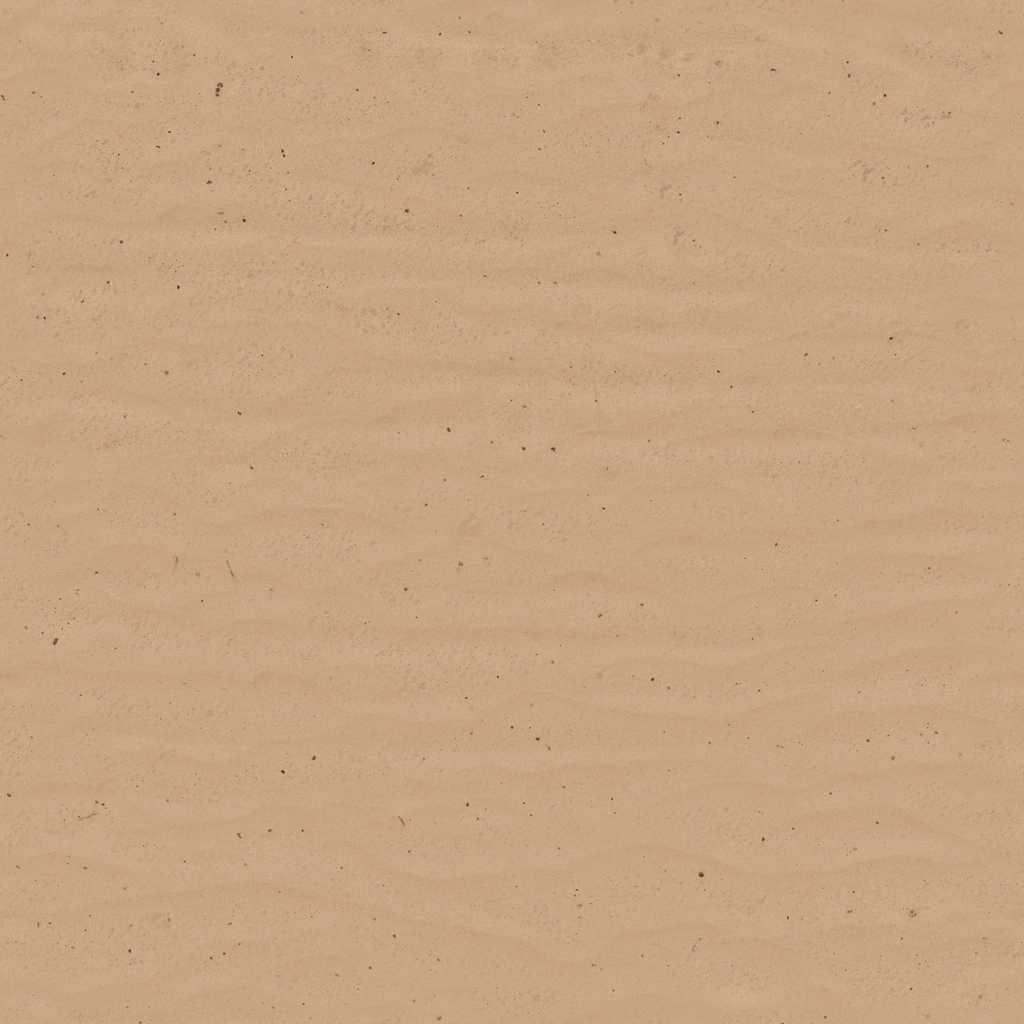
- assets/coastal-breaker-ocean/sand-base.jpg
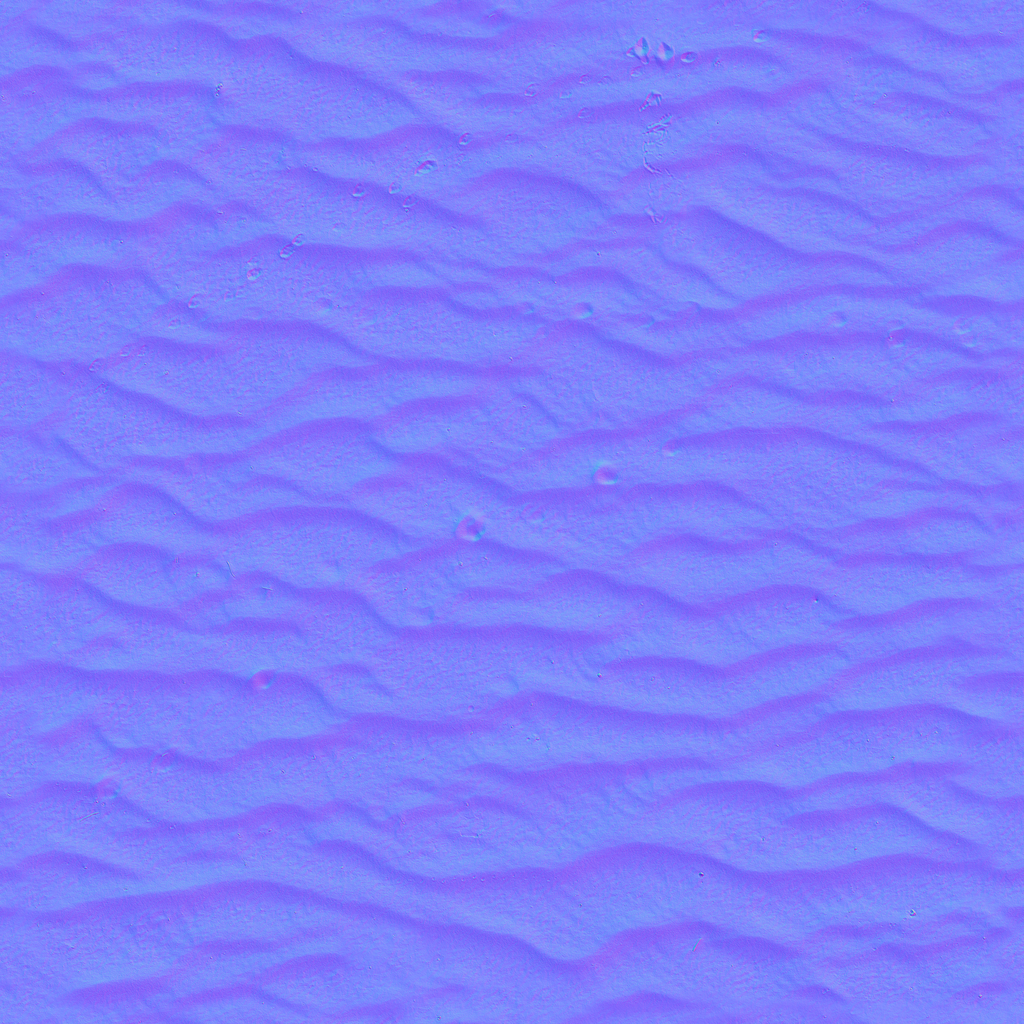
- assets/coastal-breaker-ocean/sand-normal.jpg
- assets/stylized-above-below-ocean/foam.webp
- assets/stylized-above-below-ocean/sand.webp
- examples/coastal-breaker-ocean/coastal-breaker-ocean.js
- examples/coastal-breaker-ocean/source/chain.js
- examples/coastal-breaker-ocean/source/coast.js
- examples/coastal-breaker-ocean/source/foam.js
- examples/coastal-breaker-ocean/source/noise.js
- examples/coastal-breaker-ocean/source/ocean.js
- examples/coastal-breaker-ocean/source/tsl.js
- examples/coastal-breaker-ocean/source/wave-field.js
- examples/hybrid-clear-water-ocean/hybrid-ocean-material.js
- examples/spectral-cascade-ocean/detail-texture.js
- examples/spectral-cascade-ocean/fft-pipeline.js
- examples/spectral-cascade-ocean/ocean-material.js
- examples/spectral-cascade-ocean/ocean-system.js
- examples/spectral-cascade-ocean/spectrum.js
- examples/stylized-above-below-ocean/stylized-ocean-material.js
- examples/submerged-snell-ocean/source/caustics.ts
- examples/submerged-snell-ocean/source/current.ts
- examples/submerged-snell-ocean/source/fft-compute.ts
- examples/submerged-snell-ocean/source/grade.ts
- examples/submerged-snell-ocean/source/interface-structure-layer.ts
- examples/submerged-snell-ocean/source/medium.ts
- examples/submerged-snell-ocean/source/noise.ts
- examples/submerged-snell-ocean/source/ocean-foam.ts
- examples/submerged-snell-ocean/source/ocean-material.ts
- examples/submerged-snell-ocean/source/ocean-skirt-geometry.ts
- examples/submerged-snell-ocean/source/ocean-spectrum.ts
- examples/submerged-snell-ocean/source/ocean-system.ts
- examples/submerged-snell-ocean/source/optical-constants.ts
- examples/submerged-snell-ocean/source/random.ts
- examples/submerged-snell-ocean/source/seabed-material.ts
- examples/submerged-snell-ocean/source/seabed-radiance.ts
- examples/submerged-snell-ocean/source/seabed-surface.ts
- examples/submerged-snell-ocean/source/sky-dome.ts
- examples/submerged-snell-ocean/source/sky-radiance.ts
- examples/submerged-snell-ocean/source/sun.ts
- examples/submerged-snell-ocean/source/wake-foam-map.ts
- examples/submerged-snell-ocean/source/wave-sim.ts
- examples/submerged-snell-ocean/underwater-snell-ocean.ts
- references/coastal-breaker-and-swash-ocean.md
- references/spectral-cascade-ocean-system.md
references/coastal-breaker-and-swash-ocean.md (verbatim)
Coastal breaker and swash ocean
Use this reference when the defining view is the transition from open water to
wet sand: shoaling waves, persistent breaker foam, a moving waterline, a thin
swash film, and dry terrain must meet without a seam. Read the
coastal-breaker-ocean example with this contract; the wave field, coast,
swash state, foam history, and sand response are one coupled system.
Contents
- System ownership
- Band-limited gravity field
- Layer comb and wave motion
- Coast representation
- Shallow-water swash chain
- Foam state
- Camera-following geometry
- Shoreline optics
- Runtime order
- Limits and failure patterns
- Diagnostics
1. System ownership
Keep these mechanisms together:
deterministic band fields
  -> moving gravity and capillary textures
  -> displaced deep-water grid
  -> signed-distance terrain and coast ribbons
  -> coast-normal shallow-water chains
  -> world-space and film-space foam history
  -> water / wet sand / dry sand optical blend
The coastal-breaker-ocean example owns every stage above. The surrounding
scene supplies a camera, the visible sky mesh, the animation delta, and the
two effect-owned sand textures. The ocean and visible sky evaluate the same
coastalSkyRadiance function and sun vector.
2. Band-limited gravity field
The gravity texture set contains five deterministic 256 × 256 half-float
RGBA fields. Their channels are:
R = height h
G = horizontal particle displacement d
B = dh/dx
A = dh/dy
Each field begins as seeded white noise in frequency space. Rotate frequency
coordinates by one of 0°, -10°, 10°, -5°, 5°, apply a narrow directional
band pass, and integrate horizontal displacement by dividing by
1 - exp(-iω) along the travel axis. The zero-frequency pole is harmless
because the band pass vanishes quadratically there.
The five fields form a geometric comb with COPY_RATIO = 0.87. Their seeds
are 12345, 23456, 34567, 45678, and 56789. Normalize height to unit
variance, normalize every displacement channel by the coarsest displacement
standard deviation, and weight comb entries proportional to 0.87^k with a
unit root-sum-square normalization.
The capillary field is an independent deterministic 256 × 256 isotropic
band pass with seed 54321, smoothing scales 2 and 6 texels, and no
horizontal displacement channel.
3. Layer comb and wave motion
The calibrated wave controls are:
const wave = {
  wavelengthMeters: 10,
  rmsAmplitudeMeters: 0.2,
  choppiness: 1.5,
  layerCount: 5,
  directionalSpreadDegrees: 40,
  directionDegrees: 0,
  dispersion: 1,
}
For gravity wavelength λ, use phase speed
sqrt(g λ / (2π)), with g = 9.81 m/s². The layer ratio is exactly:
LAYER_RATIO = (0.68^7 / 0.87^4)^(1/4)
Normalize layer amplitudes by the root-sum-square of all active
LAYER_RATIO^i weights so changing layer count changes comb density rather
than total variance. The eight possible direction offsets are
[0, 0.9, -0.75, 0.45, -0.35, 0.7, -1, 0.2] times the directional spread.
Capillary phase speed uses
sqrt(g/k + 7.4e-5 k) with k = 2π/λ. The three isotropic angles are
0.4, -0.8, and 1.7 radians; three aligned bands use spread fractions
0, 0.45, and -0.35. Their wavelength scales are 1, 0.72, and
0.52 from the 0.5 m base ripple scale.
4. Coast representation
The static coastline has three synchronized representations:
- an arclength-resampled mainland table with
2048entries at0.8 m; - a clockwise
96-column island loop; - a
512 × 512half-float signed-distance field covering±384 m.
Land is the positive signed-distance side. Terrain height is:
terrainHeight(xz) = clamp(0.15 * coastSDF(xz), -seaDepth, 3 m)
Outside the baked field, blend toward the far-field mainland line
x - 10 m. The mainland table extends along its endpoint tangents so a
camera-following ribbon does not terminate at the table edge.
Do not replace the coast-normal table with nearest SDF gradients. The swash columns need stable arclength ordering and stable landward normals; filtered SDF gradients alone do not provide either.
5. Shallow-water swash chain
The moving waterline is a heightless Lagrangian film with 256 coast columns
and 64 nodes per column. Mainland columns 0…159 cover a camera-following
160 m window; columns 160…255 wrap around the island.
The junction depth is REST_DEPTH = 0.25 m. With beach slope 0.15, the
rest junction is -0.25 / 0.15 m from the static shoreline. Every segment
conserves its triangular-wedge rest volume. For current segment length L,
surface level is:
eta = terrain(midpoint) + restVolume / L + shockViscosity
acceleration = -9.81 * d(eta)/dx
Use four substeps, friction 0.3, quadratic compression viscosity 0.25,
acceleration cap 25 m/s², velocity cap 6 m/s, and viscosity cap 0.5 m.
The driving sea level is low-pass filtered with a 1 s time constant and its
speed is capped at 5 m/s.
A linear spring chain is a failure: uniformly spaced nodes can balance while the water piles up. Conserved segment volume makes a flat free surface the unique equilibrium.
6. Foam state
Run two persistent ping-pong simulations:
world foam   512 × 512 over a camera-following ±80 m square
film foam    128 × 256 over coast-normal distance and coast column
The world field generates from horizontal-displacement Jacobian compression and shallow crest height. The film field generates from swash-chain compression, masks beyond the moving tip, and accelerates decay where water is swallowed back seaward. Both retain a smoothed generation pair alongside the accumulated red/green lifetime pair.
The display pattern is deterministic seed 777: bubble-raft web noise at
scales 2/6, clumping at 3/9, and fine breakup at 1/2.5. Keep the
simulation field continuous; threshold the display pattern only during
shading.
7. Camera-following geometry
The deep grid is 512 × 512 cells with a 0.4 m linear cell size for the
first 160 cells from center and 1.12 geometric growth afterward. Snap its
origin to 0.4 m world increments. The material mirrors this warp with a
linear radius of 64 m and growth 1.08 for shading footprint estimates.
The mainland and island ribbons are separate meshes. Their material coordinates carry coast column, swash distance, and local cell width; the vertex shader reconstructs world position from the coast tables and chain state. Keep the deep grid, ribbons, island loop, and land mesh in the same depth-writing render sequence.
8. Shoreline optics
Blend sand and water by the actual vertical water column:
column = max(surfaceY - terrainY, 0)
waterMask = smoothstep(0.025 m, 0.09 m, column)
The sand tiles every 3 m. Fade tangent-space normal detail from derivative
footprint once a pixel covers multiple texels. Under water, refract toward the
bed with index ratio 0.752, apply Beer-Lambert transmission
exp(-vec3(0.25, 0.04, 0.02) * pathLength), and focus two moving capillary
samples into caustic webbing. Above the water, retain dry-sand diffuse response.
Foam is a final material identity over both branches. World foam dominates offshore; film foam is parameterized along the swash chain and persists over wet sand. A detached screen-space shoreline decal cannot reproduce this ownership.
9. Runtime order
Per frame, preserve this order:
advance gravity and capillary copy phases
sample the previous completed layer cache to drive swash chains
update coast-relative chain state and data textures
update ocean uniforms and the next layer cache
render gravity and capillary composition targets
advance both foam ping-pong targets when delta > 0
render the sky and ocean scene
The one-frame completed-layer handoff into the swash driver is intentional. Reordering it creates a split CPU/GPU wave state at the junction.
10. Limits and failure patterns
- The wave field is a deterministic directional band comb, not an FFT sea-state spectrum; route ocean-scale spectral synthesis to the cascade examples.
- The swash chain is heightless. It moves the surface and waterline but does not solve a full two-dimensional shallow-water height field.
- The baked coast is finite; its far-field mainland fallback must remain straight and compatible with the arclength table endpoints.
- Rebuilding foam from the current frame loses breaker streak lifetime.
- Sampling sand normals without derivative filtering sparkles at grazing range.
- Letting the orbit camera pass below the terrain exposes the ribbon skirts and invalidates the intended view.
11. Diagnostics
The example exposes:
final       coupled ocean, swash, foam, and sand
normals     resolved water and terrain normals
foam        red = world accumulation, green = film accumulation, blue = display mask
shoreline   signed coast side plus the zero-distance band
wireframe   deep grid, mainland ribbon, island ribbon, and land topology
Use a fixed camera at (-16.2400, 3.5806, 11.1104) m, looking at the origin,
with 60° vertical field of view for deterministic coast comparisons.
Back to scottstts/Threejs-Awesome-Graphics-Agent-Skills or Agent skills.