timesfm-forecasting skill (K-Dense scientific-agent-skills)
- Install
- SKILL.md (verbatim)
- Overview
- When to Use This Skill
- ⚠️ Mandatory Preflight: System Requirements Check
- Hardware Requirements by Model Version
- 🔧 Installation
- Step 1: Verify System (always first)
- Step 2: Install TimesFM
- Step 3: Install PyTorch for Your Hardware
- Step 4: Verify Installation
- 🎯 Quick Start
- Minimal Example (5 Lines)
- Forecast from CSV
- Forecast with Covariates (XReg)
- Anomaly Detection (via Quantile Intervals)
- Output, Configuration, Workflows, and Tuning
- 🔗 Integration with Other Skills
- With statsmodels
- With matplotlib / scientific-visualization
- With exploratory-data-analysis
- 📚 Available Scripts
- scripts/checksystem.py
- scripts/forecastcsv.py
- 📖 Reference Documentation
- Common Pitfalls
- Model Versions
- Resources
- Other files in this skill
- examples/global-temperature/README.md (verbatim)
- Executive Summary
- Input Data
- Historical Temperature Anomalies (2022-2024)
- Raw Forecast Output
- Point Forecast and Confidence Intervals
- JSON Output
- Visualization
- Findings
- Key Observations
- Limitations
- Recommendations
- Reproducibility
- Files
- How to Reproduce
- Technical Notes
- API Discovery
- TimesFM 2.5 PyTorch Issue
- references/apireference.md (verbatim)
- Model Classes
- timesfm.TimesFM2p5200Mtorch
- timesfm.ForecastConfig
- Parameter Details
- Available Model Checkpoints
- Output Shape Reference
- Error Handling
- references/datapreparation.md (verbatim)
- Input Format
- Key Properties
- Loading from Common Formats
- CSV — Single Series (Long Format)
- CSV — Multiple Series (Wide Format)
- CSV — Long Format with ID Column
- Pandas DataFrame
- Numpy Arrays
- Excel
- Parquet
- JSON
- NaN Handling
- Leading NaNs
- Internal NaNs
- Trailing NaNs
- Best Practice
- Context Length Considerations
- Covariates (XReg)
- Types of Covariates
- Preparing Covariates
- XReg Modes
- Common Data Issues
- Issue: Series too short
- Issue: Series with constant values
- Issue: Extreme outliers
- Issue: Mixed frequencies in batch
- references/examplesandvalidation.md (verbatim)
- Examples
- Running the Examples
- Expected Outputs
- Quality Checklist
- Common Mistakes
- Validation & Verification
- references/outputandconfig.md (verbatim)
- 📊 Understanding the Output
- Quantile Forecast Structure
- Extracting Prediction Intervals
- 🔧 ForecastConfig Reference
- references/performancetuning.md (verbatim)
- ⚙️ Performance Tuning
- GPU Acceleration
- Batch Size Tuning
- Memory-Constrained Environments
- references/workflows.md (verbatim)
- 📋 Common Workflows
- Workflow 1: Single Series Forecast
- Workflow 2: Batch Forecasting (Many Series)
- Workflow 3: Evaluate Forecast Accuracy
What it does. Zero-shot time series forecasting with Google's TimesFM foundation model. Use for any univariate time series (sales, sensors, energy, vitals, weather) without training a custom model. Supports CSV/DataFrame/array inputs with point forecasts and prediction intervals. Includes a preflight system checker script to verify RAM/GPU before first use. Part of K-Dense-AI/scientific-agent-skills (AI Scientist skills) (K-Dense-AI/scientific-agent-skills).
| Upstream | K-Dense-AI/scientific-agent-skills |
| Skill file | skills/timesfm-forecasting/SKILL.md |
| License | MIT |
| Author | K-Dense Inc. |
| Fetched | 2026-09-10 |
Install
npx skills add K-Dense-AI/scientific-agent-skills --skill timesfm-forecasting, or copy the skill folder into~/.claude/skills/timesfm-forecasting/.- Raw file:
curl -sL https://raw.githubusercontent.com/K-Dense-AI/scientific-agent-skills/HEAD/skills/timesfm-forecasting/SKILL.md
SKILL.md (verbatim)
name: timesfm-forecasting
description: Zero-shot time series forecasting with Google's TimesFM foundation model. Use for any univariate time series (sales, sensors, energy, vitals, weather) without training a custom model. Supports CSV/DataFrame/array inputs with point forecasts and prediction intervals. Includes a preflight system checker script to verify RAM/GPU before first use.
allowed-tools: Read Write Edit Bash
license: Apache-2.0 license
metadata:
  version: "1.2"
  skill-author: Clayton Young / Superior Byte Works, LLC (@borealBytes)
  skill-version: 1.0.0
TimesFM Forecasting
Overview
TimesFM (Time Series Foundation Model) is a pretrained decoder-only foundation model developed by Google Research for time-series forecasting. It works zero-shot — feed it any univariate time series and it returns point forecasts with calibrated quantile prediction intervals, no training required.
This skill wraps TimesFM for safe, agent-friendly local inference. It includes a mandatory preflight system checker that verifies RAM, GPU memory, and disk space before the model is ever loaded so the agent never crashes a user's machine.
Key numbers: TimesFM 2.5 uses 200M parameters (~800 MB on disk, ~1.5 GB in RAM on CPU, ~1 GB VRAM on GPU). The archived v1/v2 500M-parameter model needs ~32 GB RAM. Always run the system checker first.
When to Use This Skill
Use this skill when:
- Forecasting any univariate time series (sales, demand, sensor, vitals, price, weather)
- You need zero-shot forecasting without training a custom model
- You want probabilistic forecasts with calibrated prediction intervals (quantiles)
- You have time series of any length (the model handles 1–16,384 context points)
- You need to batch-forecast hundreds or thousands of series efficiently
- You want a foundation model approach instead of hand-tuning ARIMA/ETS parameters
Do not use this skill when:
- You need classical statistical models with coefficient interpretation → use
statsmodels - You need time series classification or clustering → use
aeon - You need multivariate vector autoregression or Granger causality → use
statsmodels - Your data is tabular (not temporal) → use
scikit-learn
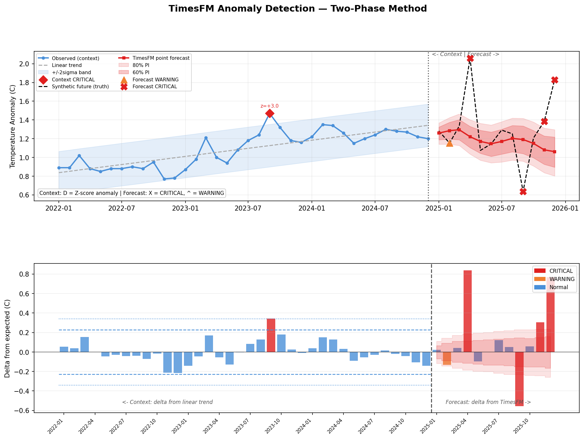
Note on Anomaly Detection: TimesFM does not have built-in anomaly detection, but you can use the quantile forecasts as prediction intervals — values outside the 90% CI (q10–q90) are statistically unusual. See the
examples/anomaly-detection/directory for a full example.
⚠️ Mandatory Preflight: System Requirements Check
CRITICAL — ALWAYS run the system checker before loading the model for the first time.
python scripts/check_system.py
This script checks:
- Available RAM — warns if below 4 GB, blocks if below 2 GB
- GPU availability — detects CUDA/MPS devices and VRAM
- Disk space — verifies room for the ~800 MB model download
- Python version — requires 3.10+
- Existing installation — checks if
timesfmandtorchare installed
Note: Model weights are NOT stored in this repository. TimesFM weights (~800 MB) download on-demand from HuggingFace on first use and cache in
~/.cache/huggingface/. The preflight checker ensures sufficient resources before any download begins.
flowchart TD
    accTitle: Preflight System Check
    accDescr: Decision flowchart showing the system requirement checks that must pass before loading TimesFM.

    start["🚀 Run check_system.py"] --> ram{"RAM ≥ 4 GB?"}
    ram -->|"Yes"| gpu{"GPU available?"}
    ram -->|"No (2-4 GB)"| warn_ram["⚠️ Warning: tight RAM<br/>CPU-only, small batches"]
    ram -->|"No (< 2 GB)"| block["🛑 BLOCKED<br/>Insufficient memory"]
    warn_ram --> disk
    gpu -->|"CUDA / MPS"| vram{"VRAM ≥ 2 GB?"}
    gpu -->|"CPU only"| cpu_ok["✅ CPU mode<br/>Slower but works"]
    vram -->|"Yes"| gpu_ok["✅ GPU mode<br/>Fast inference"]
    vram -->|"No"| cpu_ok
    gpu_ok --> disk{"Disk ≥ 2 GB free?"}
    cpu_ok --> disk
    disk -->|"Yes"| ready["✅ READY<br/>Safe to load model"]
    disk -->|"No"| block_disk["🛑 BLOCKED<br/>Need space for weights"]

    classDef ok fill:#dcfce7,stroke:#16a34a,stroke-width:2px,color:#14532d
    classDef warn fill:#fef9c3,stroke:#ca8a04,stroke-width:2px,color:#713f12
    classDef block fill:#fee2e2,stroke:#dc2626,stroke-width:2px,color:#7f1d1d
    classDef neutral fill:#f3f4f6,stroke:#6b7280,stroke-width:2px,color:#1f2937

    class ready,gpu_ok,cpu_ok ok
    class warn_ram warn
    class block,block_disk block
    class start,ram,gpu,vram,disk neutral
Hardware Requirements by Model Version
| Model | Parameters | RAM (CPU) | VRAM (GPU) | Disk | Context |
|---|---|---|---|---|---|
| TimesFM 2.5 (recommended) | 200M | ≥ 4 GB | ≥ 2 GB | ~800 MB | up to 16,384 |
| TimesFM 2.0 (archived) | 500M | ≥ 16 GB | ≥ 8 GB | ~2 GB | up to 2,048 |
| TimesFM 1.0 (archived) | 200M | ≥ 8 GB | ≥ 4 GB | ~800 MB | up to 2,048 |
Recommendation: Always use TimesFM 2.5 unless you have a specific reason to use an older checkpoint. It is smaller, faster, and supports 8× longer context.
🔧 Installation
Step 1: Verify System (always first)
python scripts/check_system.py
Step 2: Install TimesFM
# Using uv (recommended by this repo)
uv pip install timesfm[torch]

# For JAX/Flax backend (faster on TPU/GPU)
uv pip install timesfm[flax]
Step 3: Install PyTorch for Your Hardware
# CUDA 12.1 (NVIDIA GPU)
uv pip install torch>=2.0.0 --index-url https://download.pytorch.org/whl/cu121

# CPU only
uv pip install torch>=2.0.0 --index-url https://download.pytorch.org/whl/cpu

# Apple Silicon (MPS)
uv pip install torch>=2.0.0  # MPS support is built-in
Step 4: Verify Installation
import timesfm
import numpy as np
print(f"TimesFM version: {timesfm.__version__}")
print("Installation OK")
🎯 Quick Start
Minimal Example (5 Lines)
import torch, numpy as np, timesfm

torch.set_float32_matmul_precision("high")

model = timesfm.TimesFM_2p5_200M_torch.from_pretrained(
    "google/timesfm-2.5-200m-pytorch"
)
model.compile(timesfm.ForecastConfig(
    max_context=1024, max_horizon=256, normalize_inputs=True,
    use_continuous_quantile_head=True, force_flip_invariance=True,
    infer_is_positive=True, fix_quantile_crossing=True,
))

point, quantiles = model.forecast(horizon=24, inputs=[
    np.sin(np.linspace(0, 20, 200)),  # any 1-D array
])
# point.shape == (1, 24)        — median forecast
# quantiles.shape == (1, 24, 10) — 10th–90th percentile bands
Forecast from CSV
import pandas as pd, numpy as np

df = pd.read_csv("monthly_sales.csv", parse_dates=["date"], index_col="date")

# Convert each column to a list of arrays
inputs = [df[col].dropna().values.astype(np.float32) for col in df.columns]

point, quantiles = model.forecast(horizon=12, inputs=inputs)

# Build a results DataFrame
for i, col in enumerate(df.columns):
    last_date = df[col].dropna().index[-1]
    future_dates = pd.date_range(last_date, periods=13, freq="MS")[1:]
    forecast_df = pd.DataFrame({
        "date": future_dates,
        "forecast": point[i],
        "lower_80": quantiles[i, :, 2],  # 20th percentile
        "upper_80": quantiles[i, :, 8],  # 80th percentile
    })
    print(f"\n--- {col} ---")
    print(forecast_df.to_string(index=False))
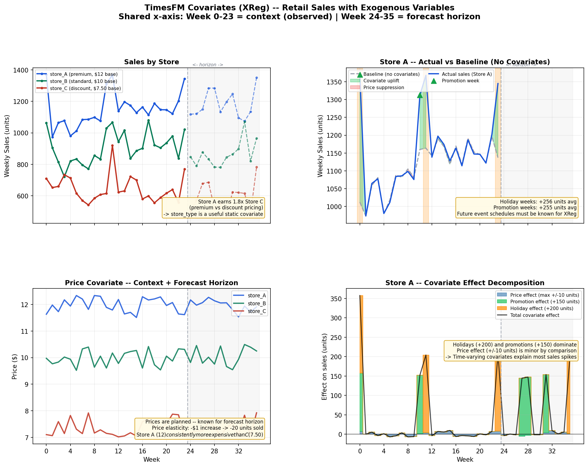
Forecast with Covariates (XReg)
TimesFM 2.5+ supports exogenous variables through forecast_with_covariates(). Requires timesfm[xreg].
# Requires: uv pip install timesfm[xreg]
point, quantiles = model.forecast_with_covariates(
    inputs=inputs,
    dynamic_numerical_covariates={"price": price_arrays},
    dynamic_categorical_covariates={"holiday": holiday_arrays},
    static_categorical_covariates={"region": region_labels},
    xreg_mode="xreg + timesfm",  # or "timesfm + xreg"
)
| Covariate Type | Description | Example |
|---|---|---|
dynamic_numerical |
Time-varying numeric | price, temperature, promotion spend |
dynamic_categorical |
Time-varying categorical | holiday flag, day of week |
static_numerical |
Per-series numeric | store size, account age |
static_categorical |
Per-series categorical | store type, region, product category |
XReg Modes:
"xreg + timesfm"(default): TimesFM forecasts first, then XReg adjusts residuals"timesfm + xreg": XReg fits first, then TimesFM forecasts residuals
See
examples/covariates-forecasting/for a complete example with synthetic retail data.
Anomaly Detection (via Quantile Intervals)
TimesFM does not have built-in anomaly detection, but the quantile forecasts naturally provide prediction intervals that can detect anomalies:
point, q = model.forecast(horizon=H, inputs=[values])

# 90% prediction interval
lower_90 = q[0, :, 1]  # 10th percentile
upper_90 = q[0, :, 9]  # 90th percentile

# Detect anomalies: values outside the 90% CI
actual = test_values  # your holdout data
anomalies = (actual < lower_90) | (actual > upper_90)

# Severity levels
is_warning = (actual < q[0, :, 2]) | (actual > q[0, :, 8])  # outside 80% CI
is_critical = anomalies  # outside 90% CI
| Severity | Condition | Interpretation |
|---|---|---|
| Normal | Inside 80% CI | Expected behavior |
| Warning | Outside 80% CI | Unusual but possible |
| Critical | Outside 90% CI | Statistically rare (< 10% probability) |
See
examples/anomaly-detection/for a complete example with visualization.
# Requires: uv pip install timesfm[xreg]
point, quantiles = model.forecast_with_covariates(
    inputs=inputs,
    dynamic_numerical_covariates={"temperature": temp_arrays},
    dynamic_categorical_covariates={"day_of_week": dow_arrays},
    static_categorical_covariates={"region": region_labels},
    xreg_mode="xreg + timesfm",  # or "timesfm + xreg"
)
Output, Configuration, Workflows, and Tuning
- references/output_and_config.md: reading the point
forecast and the 10 quantile bands, deriving prediction intervals, and every
ForecastConfigfield. - references/workflows.md: the standard forecast sequence, many-series forecasting from a wide CSV, and backtesting with interval coverage.
- references/performance_tuning.md: GPU and TF32
setup,
per_core_batch_sizeby available memory, and memory management. - references/examples_and_validation.md: runnable examples, the quality checklist, common mistakes, and regression checks.
🔗 Integration with Other Skills
With statsmodels
Use statsmodels for classical models (ARIMA, SARIMAX) as a comparison baseline:
# TimesFM forecast
tfm_point, tfm_q = model.forecast(horizon=H, inputs=[values])

# statsmodels ARIMA forecast
from statsmodels.tsa.arima.model import ARIMA
arima = ARIMA(values, order=(1,1,1)).fit()
arima_forecast = arima.forecast(steps=H)

# Compare
print(f"TimesFM MAE: {np.mean(np.abs(actual - tfm_point[0])):.2f}")
print(f"ARIMA MAE:   {np.mean(np.abs(actual - arima_forecast)):.2f}")
With matplotlib / scientific-visualization
Plot forecasts with prediction intervals as publication-quality figures.
With exploratory-data-analysis
Run EDA on the time series before forecasting to understand trends, seasonality, and stationarity.
📚 Available Scripts
scripts/check_system.py
Mandatory preflight checker. Run before first model load.
python scripts/check_system.py
Output example:
=== TimesFM System Requirements Check ===

[RAM]       Total: 32.0 GB | Available: 24.3 GB  ✅ PASS
[GPU]       NVIDIA RTX 4090 | VRAM: 24.0 GB      ✅ PASS
[Disk]      Free: 142.5 GB                        ✅ PASS
[Python]    3.12.1                                 ✅ PASS
[timesfm]   Installed (2.5.0)                      ✅ PASS
[torch]     Installed (2.4.1+cu121)                ✅ PASS

VERDICT: ✅ System is ready for TimesFM 2.5 (GPU mode)
Recommended: per_core_batch_size=128
scripts/forecast_csv.py
End-to-end CSV forecasting with automatic system check.
python scripts/forecast_csv.py input.csv \
    --horizon 24 \
    --date-col date \
    --value-cols sales,revenue \
    --output forecasts.csv
📖 Reference Documentation
Detailed guides in references/:
| File | Contents |
|---|---|
references/system_requirements.md |
Hardware tiers, GPU/CPU selection, memory estimation formulas |
references/api_reference.md |
Full ForecastConfig docs, from_pretrained options, output shapes |
references/data_preparation.md |
Input formats, NaN handling, CSV loading, covariate setup |
Common Pitfalls
- Not running system check → model load crashes on low-RAM machines. Always run
check_system.pyfirst. - Forgetting
model.compile()→RuntimeError: Model is not compiled. Must callcompile()beforeforecast(). - Not setting
normalize_inputs=True→ unstable forecasts for series with large values. - Using v1/v2 on machines with < 32 GB RAM → use TimesFM 2.5 (200M params) instead.
- Not setting
fix_quantile_crossing=True→ quantiles may not be monotonic (q10 > q50). - Huge
per_core_batch_sizeon small GPU → CUDA OOM. Start small, increase. - Passing 2-D arrays → TimesFM expects a list of 1-D arrays, not a 2-D matrix.
- Forgetting
torch.set_float32_matmul_precision("high")→ slower inference on Ampere+ GPUs. - Not handling NaN in output → edge cases with very short series. Always check
np.isnan(point).any(). - Using
infer_is_positive=Truefor series that can be negative → clamps forecasts at zero. Set False for temperature, returns, etc.
Model Versions
timeline
    accTitle: TimesFM Version History
    accDescr: Timeline of TimesFM model releases showing parameter counts and key improvements.

    section 2024
        TimesFM 1.0 : 200M params, 2K context, JAX only
        TimesFM 2.0 : 500M params, 2K context, PyTorch + JAX
    section 2025
        TimesFM 2.5 : 200M params, 16K context, quantile head, no frequency indicator
| Version | Params | Context | Quantile Head | Frequency Flag | Status |
|---|---|---|---|---|---|
| 2.5 | 200M | 16,384 | ✅ Continuous (30M) | ❌ Removed | Latest |
| 2.0 | 500M | 2,048 | ✅ Fixed buckets | ✅ Required | Archived |
| 1.0 | 200M | 2,048 | ✅ Fixed buckets | ✅ Required | Archived |
Hugging Face checkpoints:
google/timesfm-2.5-200m-pytorch(recommended)google/timesfm-2.5-200m-flaxgoogle/timesfm-2.0-500m-pytorch(archived)google/timesfm-1.0-200m-pytorch(archived)
Resources
- Paper: A Decoder-Only Foundation Model for Time-Series Forecasting (ICML 2024)
- Repository: https://github.com/google-research/timesfm
- Hugging Face: https://huggingface.co/collections/google/timesfm-release-66e4be5fdb56e960c1e482a6
- Google Blog: https://research.google/blog/a-decoder-only-foundation-model-for-time-series-forecasting/
- BigQuery Integration: https://cloud.google.com/bigquery/docs/timesfm-model
Other files in this skill
- examples/anomaly-detection/detect_anomalies.py
- examples/anomaly-detection/output/anomaly_detection.json
- examples/anomaly-detection/output/anomaly_detection.png
- examples/covariates-forecasting/demo_covariates.py
- examples/covariates-forecasting/output/covariates_data.png
- examples/covariates-forecasting/output/covariates_metadata.json
- examples/covariates-forecasting/output/sales_with_covariates.csv
- examples/global-temperature/README.md
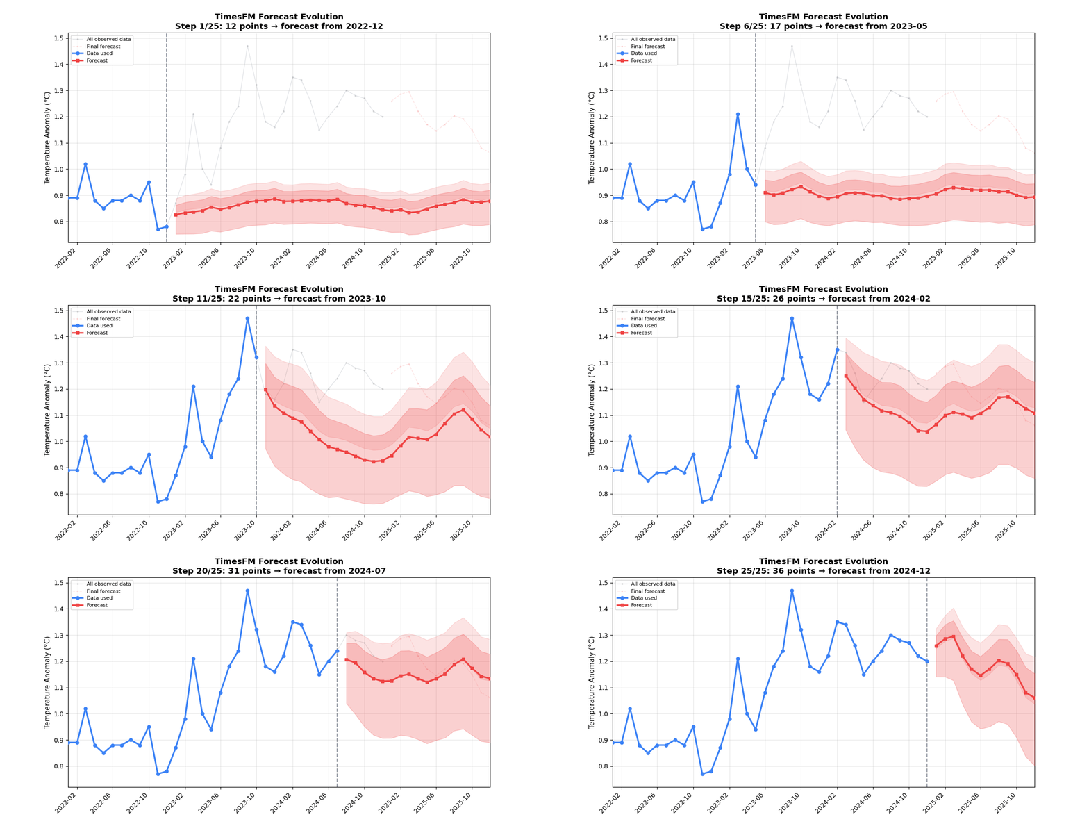
- examples/global-temperature/generate_animation_data.py
- examples/global-temperature/generate_gif.py
- examples/global-temperature/generate_html.py
- examples/global-temperature/output/animation_data.json
- examples/global-temperature/output/forecast_animation.gif
- examples/global-temperature/output/forecast_output.csv
- examples/global-temperature/output/forecast_output.json
- examples/global-temperature/output/forecast_visualization.png
- examples/global-temperature/output/interactive_forecast.html
- examples/global-temperature/run_example.sh
- examples/global-temperature/run_forecast.py
- examples/global-temperature/temperature_anomaly.csv
- examples/global-temperature/visualize_forecast.py
- references/api_reference.md
- references/data_preparation.md
- references/examples_and_validation.md
- references/output_and_config.md
- references/performance_tuning.md
- references/system_requirements.md
- references/workflows.md
- scripts/check_system.py
- scripts/forecast_csv.py
examples/global-temperature/README.md (verbatim)
TimesFM Forecast Report: Global Temperature Anomaly (2025)
Model: TimesFM 1.0 (200M) PyTorch
Generated: 2026-02-21
Source: NOAA GISTEMP Global Land-Ocean Temperature Index
Executive Summary
TimesFM forecasts a mean temperature anomaly of 1.19°C for 2025, slightly below the 2024 average of 1.25°C. The model predicts continued elevated temperatures with a peak of 1.30°C in March 2025 and a minimum of 1.06°C in December 2025.
Input Data
Historical Temperature Anomalies (2022-2024)
| Date | Anomaly (°C) | Date | Anomaly (°C) | Date | Anomaly (°C) |
|---|---|---|---|---|---|
| 2022-01 | 0.89 | 2023-01 | 0.87 | 2024-01 | 1.22 |
| 2022-02 | 0.89 | 2023-02 | 0.98 | 2024-02 | 1.35 |
| 2022-03 | 1.02 | 2023-03 | 1.21 | 2024-03 | 1.34 |
| 2022-04 | 0.88 | 2023-04 | 1.00 | 2024-04 | 1.26 |
| 2022-05 | 0.85 | 2023-05 | 0.94 | 2024-05 | 1.15 |
| 2022-06 | 0.88 | 2023-06 | 1.08 | 2024-06 | 1.20 |
| 2022-07 | 0.88 | 2023-07 | 1.18 | 2024-07 | 1.24 |
| 2022-08 | 0.90 | 2023-08 | 1.24 | 2024-08 | 1.30 |
| 2022-09 | 0.88 | 2023-09 | 1.47 | 2024-09 | 1.28 |
| 2022-10 | 0.95 | 2023-10 | 1.32 | 2024-10 | 1.27 |
| 2022-11 | 0.77 | 2023-11 | 1.18 | 2024-11 | 1.22 |
| 2022-12 | 0.78 | 2023-12 | 1.16 | 2024-12 | 1.20 |
Statistics:
- Total observations: 36 months
- Mean anomaly: 1.09°C
- Trend (2022→2024): +0.37°C
Raw Forecast Output
Point Forecast and Confidence Intervals
| Month | Point | 80% CI | 90% CI |
|---|---|---|---|
| 2025-01 | 1.259 | [1.141, 1.297] | [1.248, 1.324] |
| 2025-02 | 1.286 | [1.141, 1.340] | [1.277, 1.375] |
| 2025-03 | 1.295 | [1.127, 1.355] | [1.287, 1.404] |
| 2025-04 | 1.221 | [1.035, 1.290] | [1.208, 1.331] |
| 2025-05 | 1.170 | [0.969, 1.239] | [1.153, 1.289] |
| 2025-06 | 1.146 | [0.942, 1.218] | [1.128, 1.270] |
| 2025-07 | 1.170 | [0.950, 1.248] | [1.151, 1.300] |
| 2025-08 | 1.203 | [0.971, 1.284] | [1.186, 1.341] |
| 2025-09 | 1.191 | [0.959, 1.283] | [1.178, 1.335] |
| 2025-10 | 1.149 | [0.908, 1.240] | [1.126, 1.287] |
| 2025-11 | 1.080 | [0.836, 1.176] | [1.062, 1.228] |
| 2025-12 | 1.061 | [0.802, 1.153] | [1.037, 1.217] |
JSON Output
{
  "model": "TimesFM 1.0 (200M) PyTorch",
  "input": {
    "source": "NOAA GISTEMP Global Temperature Anomaly",
    "n_observations": 36,
    "date_range": "2022-01 to 2024-12",
    "mean_anomaly_c": 1.089
  },
  "forecast": {
    "horizon": 12,
    "dates": ["2025-01", "2025-02", "2025-03", "2025-04", "2025-05", "2025-06",
              "2025-07", "2025-08", "2025-09", "2025-10", "2025-11", "2025-12"],
    "point": [1.259, 1.286, 1.295, 1.221, 1.170, 1.146, 1.170, 1.203, 1.191, 1.149, 1.080, 1.061]
  },
  "summary": {
    "forecast_mean_c": 1.186,
    "forecast_max_c": 1.295,
    "forecast_min_c": 1.061,
    "vs_last_year_mean": -0.067
  }
}
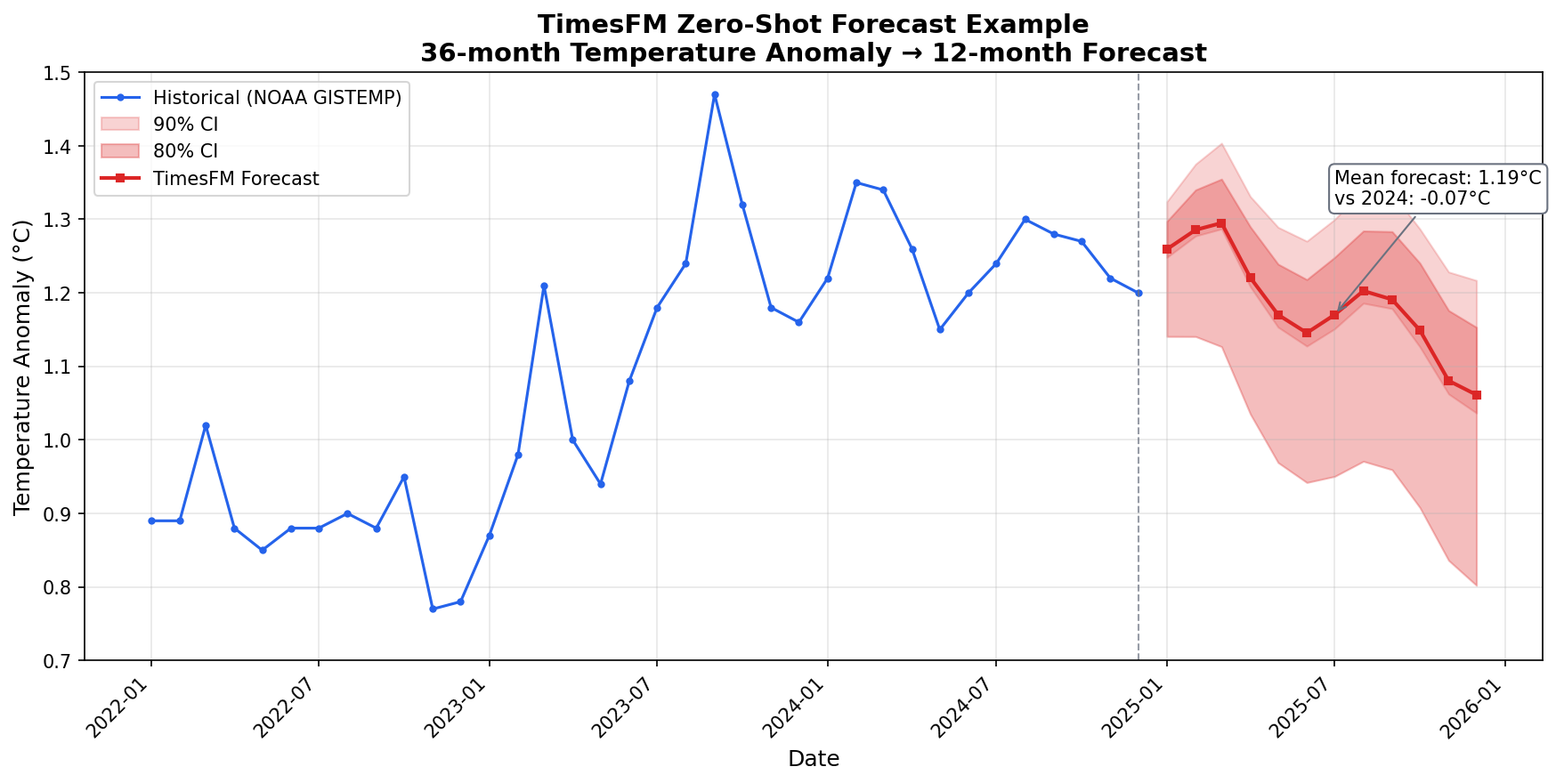
Visualization
Temperature Anomaly Forecast
Findings
Key Observations
Slight cooling trend expected: The model forecasts a mean anomaly 0.07°C below 2024 levels, suggesting a potential stabilization after the record-breaking temperatures of 2023-2024.
Seasonal pattern preserved: The forecast shows the expected seasonal variation with higher anomalies in late winter (Feb-Mar) and lower in late fall (Nov-Dec).
Widening uncertainty: The 90% CI expands from ±0.04°C in January to ±0.08°C in December, reflecting typical forecast uncertainty growth over time.
Peak temperature: March 2025 is predicted to have the highest anomaly at 1.30°C, potentially approaching the September 2023 record of 1.47°C.
Limitations
- TimesFM is a zero-shot forecaster without physical climate model constraints
- The 36-month training window may not capture multi-decadal climate trends
- El Niño/La Niña cycles are not explicitly modeled
Recommendations
- Use this forecast as a baseline comparison for physics-based climate models
- Update forecast quarterly as new observations become available
- Consider ensemble approaches combining TimesFM with other methods
Reproducibility
Files
| File | Description |
|---|---|
temperature_anomaly.csv |
Input data (36 months) |
forecast_output.csv |
Point forecast with quantiles |
forecast_output.json |
Machine-readable forecast |
forecast_visualization.png |
Fan chart visualization |
run_forecast.py |
Forecasting script |
visualize_forecast.py |
Visualization script |
run_example.sh |
One-click runner |
How to Reproduce
# Install dependencies
uv pip install "timesfm[torch]" matplotlib pandas numpy

# Run the complete example
cd skills/timesfm-forecasting/examples/global-temperature
./run_example.sh
Technical Notes
API Discovery
The TimesFM PyTorch API differs from the GitHub README documentation:
Documented (GitHub README):
model = timesfm.TimesFm(
    context_len=512,
    horizon_len=128,
    backend="gpu",
)
model.load_from_google_repo("google/timesfm-2.5-200m-pytorch")
Actual Working API:
hparams = timesfm.TimesFmHparams(horizon_len=12)
checkpoint = timesfm.TimesFmCheckpoint(
    huggingface_repo_id="google/timesfm-1.0-200m-pytorch"
)
model = timesfm.TimesFm(hparams=hparams, checkpoint=checkpoint)
TimesFM 2.5 PyTorch Issue
The google/timesfm-2.5-200m-pytorch checkpoint downloads as model.safetensors, but the TimesFM loader expects torch_model.ckpt. This causes a FileNotFoundError at model load time. Using TimesFM 1.0 PyTorch resolves this issue.
Report generated by TimesFM Forecasting Skill (scientific-agent-skills)
references/api_reference.md (verbatim)
TimesFM API Reference
Model Classes
timesfm.TimesFM_2p5_200M_torch
The primary model class for TimesFM 2.5 (200M parameters, PyTorch backend).
from_pretrained()
model = timesfm.TimesFM_2p5_200M_torch.from_pretrained(
    "google/timesfm-2.5-200m-pytorch",
    cache_dir=None,         # Optional: custom cache directory
    force_download=True,    # Re-download even if cached
)
| Parameter | Type | Default | Description |
|---|---|---|---|
model_id |
str | "google/timesfm-2.5-200m-pytorch" |
Hugging Face model ID |
revision |
str | None | None | Specific model revision |
cache_dir |
str | Path | None | None | Custom cache directory |
force_download |
bool | True | Force re-download of weights |
Returns: Initialized TimesFM_2p5_200M_torch instance (not yet compiled).
compile()
Compiles the model with the given forecast configuration. Must be called before forecast().
model.compile(
    timesfm.ForecastConfig(
        max_context=1024,
        max_horizon=256,
        normalize_inputs=True,
        per_core_batch_size=32,
        use_continuous_quantile_head=True,
        force_flip_invariance=True,
        infer_is_positive=True,
        fix_quantile_crossing=True,
    )
)
Raises: Nothing (but forecast() will raise RuntimeError if not compiled).
forecast()
Run inference on one or more time series.
point_forecast, quantile_forecast = model.forecast(
    horizon=24,
    inputs=[array1, array2, ...],
)
| Parameter | Type | Description |
|---|---|---|
horizon |
int | Number of future steps to forecast |
inputs |
list[np.ndarray] | List of 1-D numpy arrays (each is a time series) |
Returns: tuple[np.ndarray, np.ndarray]
point_forecast: shape(batch_size, horizon)— median (0.5 quantile)quantile_forecast: shape(batch_size, horizon, 10)— [mean, q10, q20, ..., q90]
Raises: RuntimeError if model is not compiled.
Key behaviors:
- Leading NaN values are stripped automatically
- Internal NaN values are linearly interpolated
- Series longer than
max_contextare truncated (lastmax_contextpoints used) - Series shorter than
max_contextare padded
forecast_with_covariates()
Run inference with exogenous variables (requires timesfm[xreg]).
point, quantiles = model.forecast_with_covariates(
    inputs=inputs,
    dynamic_numerical_covariates={"temp": [temp_array1, temp_array2]},
    dynamic_categorical_covariates={"dow": [dow_array1, dow_array2]},
    static_categorical_covariates={"region": ["east", "west"]},
    xreg_mode="xreg + timesfm",
)
| Parameter | Type | Description |
|---|---|---|
inputs |
list[np.ndarray] | Target time series |
dynamic_numerical_covariates |
dict[str, list[np.ndarray]] | Time-varying numeric features |
dynamic_categorical_covariates |
dict[str, list[np.ndarray]] | Time-varying categorical features |
static_categorical_covariates |
dict[str, list[str]] | Fixed categorical features per series |
xreg_mode |
str | "xreg + timesfm" or "timesfm + xreg" |
Note: Dynamic covariates must have length context + horizon for each series.
timesfm.ForecastConfig
Immutable dataclass controlling all forecast behavior.
@dataclasses.dataclass(frozen=True)
class ForecastConfig:
    max_context: int = 0
    max_horizon: int = 0
    normalize_inputs: bool = False
    per_core_batch_size: int = 1
    use_continuous_quantile_head: bool = False
    force_flip_invariance: bool = True
    infer_is_positive: bool = True
    fix_quantile_crossing: bool = False
    return_backcast: bool = False
    quantiles: list[float] = [0.1, 0.2, 0.3, 0.4, 0.5, 0.6, 0.7, 0.8, 0.9]
    decode_index: int = 5
Parameter Details
max_context (int, default=0)
Maximum number of historical time points to use as context.
- 0: Use the model's maximum supported context (16,384 for v2.5)
- N: Truncate series to last N points
- Best practice: Set to the length of your longest series, or 512–2048 for speed
max_horizon (int, default=0)
Maximum forecast horizon.
- 0: Use the model's maximum
- N: Forecasts up to N steps (can still call
forecast(horizon=M)where M ≤ N) - Best practice: Set to your expected maximum forecast length
normalize_inputs (bool, default=False)
Whether to z-normalize each series before feeding to the model.
- True (RECOMMENDED): Normalizes each series to zero mean, unit variance
- False: Raw values are passed directly
- When False is OK: Only if your series are already normalized or very close to scale 1.0
per_core_batch_size (int, default=1)
Number of series processed per device in each batch.
- Increase for throughput, decrease if OOM
- See
references/system_requirements.mdfor recommended values by hardware
use_continuous_quantile_head (bool, default=False)
Use the 30M-parameter continuous quantile head for better interval calibration.
- True (RECOMMENDED): More accurate prediction intervals, especially for longer horizons
- False: Uses fixed quantile buckets (faster but less accurate intervals)
force_flip_invariance (bool, default=True)
Ensures the model satisfies f(-x) = -f(x).
- True (RECOMMENDED): Mathematical consistency — forecasts are invariant to sign flip
- False: Slightly faster but may produce asymmetric forecasts
infer_is_positive (bool, default=True)
Automatically detect if all input values are positive and clamp forecasts ≥ 0.
- True: Safe for sales, demand, counts, prices, volumes
- False: Required for temperature, returns, PnL, any series that can be negative
fix_quantile_crossing (bool, default=False)
Post-process quantiles to ensure monotonicity (q10 ≤ q20 ≤ ... ≤ q90).
- True (RECOMMENDED): Guarantees well-ordered quantiles
- False: Slightly faster but quantiles may occasionally cross
return_backcast (bool, default=False)
Return the model's reconstruction of the input (backcast) in addition to forecast.
- True: Used for covariate workflows and diagnostics
- False: Only return forecast
Available Model Checkpoints
| Model ID | Version | Params | Backend | Context |
|---|---|---|---|---|
google/timesfm-2.5-200m-pytorch |
2.5 | 200M | PyTorch | 16,384 |
google/timesfm-2.5-200m-flax |
2.5 | 200M | JAX/Flax | 16,384 |
google/timesfm-2.5-200m-transformers |
2.5 | 200M | Transformers | 16,384 |
google/timesfm-2.0-500m-pytorch |
2.0 | 500M | PyTorch | 2,048 |
google/timesfm-2.0-500m-jax |
2.0 | 500M | JAX | 2,048 |
google/timesfm-1.0-200m-pytorch |
1.0 | 200M | PyTorch | 2,048 |
google/timesfm-1.0-200m |
1.0 | 200M | JAX | 2,048 |
Output Shape Reference
| Output | Shape | Description |
|---|---|---|
point_forecast |
(B, H) |
Median forecast for B series, H steps |
quantile_forecast |
(B, H, 10) |
Full quantile distribution |
quantile_forecast[:,:,0] |
(B, H) |
Mean |
quantile_forecast[:,:,1] |
(B, H) |
10th percentile |
quantile_forecast[:,:,5] |
(B, H) |
50th percentile (= point_forecast) |
quantile_forecast[:,:,9] |
(B, H) |
90th percentile |
Where B = batch size (number of input series), H = forecast horizon.
Error Handling
| Error | Cause | Fix |
|---|---|---|
RuntimeError: Model is not compiled |
Called forecast() before compile() |
Call model.compile(ForecastConfig(...)) first |
torch.cuda.OutOfMemoryError |
Batch too large for GPU | Reduce per_core_batch_size |
ValueError: inputs must be list |
Passed array instead of list | Wrap in list: [array] |
HfHubHTTPError |
Download failed | Check internet, set HF_HOME to writable dir |
references/data_preparation.md (verbatim)
Data Preparation for TimesFM
Input Format
TimesFM accepts a list of 1-D numpy arrays. Each array represents one univariate time series.
inputs = [
    np.array([1.0, 2.0, 3.0, 4.0, 5.0]),       # Series 1
    np.array([10.0, 20.0, 15.0, 25.0]),          # Series 2 (different length)
    np.array([100.0, 110.0, 105.0, 115.0, 120.0, 130.0]),  # Series 3
]
Key Properties
- Variable lengths: Series in the same batch can have different lengths
- Float values: Use
np.float32ornp.float64 - 1-D only: Each array must be 1-dimensional (not 2-D matrix rows)
- NaN handling: Leading NaNs are stripped; internal NaNs are linearly interpolated
Loading from Common Formats
CSV — Single Series (Long Format)
import pandas as pd
import numpy as np

df = pd.read_csv("data.csv", parse_dates=["date"])
values = df["value"].values.astype(np.float32)
inputs = [values]
CSV — Multiple Series (Wide Format)
df = pd.read_csv("data.csv", parse_dates=["date"], index_col="date")
inputs = [df[col].dropna().values.astype(np.float32) for col in df.columns]
CSV — Long Format with ID Column
df = pd.read_csv("data.csv", parse_dates=["date"])
inputs = []
for series_id, group in df.groupby("series_id"):
    values = group.sort_values("date")["value"].values.astype(np.float32)
    inputs.append(values)
Pandas DataFrame
# Single column
inputs = [df["temperature"].values.astype(np.float32)]

# Multiple columns
inputs = [df[col].dropna().values.astype(np.float32) for col in numeric_cols]
Numpy Arrays
# 2-D array (rows = series, cols = time steps)
data = np.load("timeseries.npy")  # shape (N, T)
inputs = [data[i] for i in range(data.shape[0])]

# Or from 1-D
inputs = [np.sin(np.linspace(0, 10, 200))]
Excel
df = pd.read_excel("data.xlsx", sheet_name="Sheet1")
inputs = [df[col].dropna().values.astype(np.float32) for col in df.select_dtypes(include=[np.number]).columns]
Parquet
df = pd.read_parquet("data.parquet")
inputs = [df[col].dropna().values.astype(np.float32) for col in df.select_dtypes(include=[np.number]).columns]
JSON
import json

with open("data.json") as f:
    data = json.load(f)

# Assumes {"series_name": [values...], ...}
inputs = [np.array(values, dtype=np.float32) for values in data.values()]
NaN Handling
TimesFM handles NaN values automatically:
Leading NaNs
Stripped before feeding to the model:
# Input:  [NaN, NaN, 1.0, 2.0, 3.0]
# Actual: [1.0, 2.0, 3.0]
Internal NaNs
Linearly interpolated:
# Input:  [1.0, NaN, 3.0, NaN, NaN, 6.0]
# Actual: [1.0, 2.0, 3.0, 4.0, 5.0, 6.0]
Trailing NaNs
Not handled — drop them before passing to the model:
values = df["value"].values.astype(np.float32)
# Remove trailing NaNs
while len(values) > 0 and np.isnan(values[-1]):
    values = values[:-1]
inputs = [values]
Best Practice
def clean_series(arr: np.ndarray) -> np.ndarray:
    """Clean a time series for TimesFM input."""
    arr = np.asarray(arr, dtype=np.float32)
    # Remove trailing NaNs
    while len(arr) > 0 and np.isnan(arr[-1]):
        arr = arr[:-1]
    # Replace inf with NaN (will be interpolated)
    arr[np.isinf(arr)] = np.nan
    return arr

inputs = [clean_series(df[col].values) for col in cols]
Context Length Considerations
| Context Length | Use Case | Notes |
|---|---|---|
| 64–256 | Quick prototyping | Minimal context, fast |
| 256–512 | Daily data, ~1 year | Good balance |
| 512–1024 | Daily data, ~2-3 years | Standard production |
| 1024–4096 | Hourly data, weekly patterns | More context = better |
| 4096–16384 | High-frequency, long patterns | TimesFM 2.5 maximum |
Rule of thumb: Provide at least 3–5 full cycles of the dominant pattern (e.g., for weekly seasonality with daily data, provide at least 21–35 days).
Covariates (XReg)
TimesFM 2.5 supports exogenous variables through the forecast_with_covariates() API.
Types of Covariates
| Type | Description | Example |
|---|---|---|
| Dynamic numerical | Time-varying numeric features | Temperature, price, promotion spend |
| Dynamic categorical | Time-varying categorical features | Day of week, holiday flag |
| Static categorical | Fixed per-series features | Store ID, region, product category |
Preparing Covariates
Each covariate must have length context + horizon for each series:
import numpy as np

context_len = 100   # length of historical data
horizon = 24        # forecast horizon
total_len = context_len + horizon

# Dynamic numerical: temperature forecast for each series
temp = [
    np.random.randn(total_len).astype(np.float32),  # Series 1
    np.random.randn(total_len).astype(np.float32),  # Series 2
]

# Dynamic categorical: day of week (0-6) for each series
dow = [
    np.tile(np.arange(7), total_len // 7 + 1)[:total_len],  # Series 1
    np.tile(np.arange(7), total_len // 7 + 1)[:total_len],  # Series 2
]

# Static categorical: one label per series
regions = ["east", "west"]

# Forecast with covariates
point, quantiles = model.forecast_with_covariates(
    inputs=[values1, values2],
    dynamic_numerical_covariates={"temperature": temp},
    dynamic_categorical_covariates={"day_of_week": dow},
    static_categorical_covariates={"region": regions},
    xreg_mode="xreg + timesfm",
)
XReg Modes
| Mode | Description |
|---|---|
"xreg + timesfm" |
Covariates processed first, then combined with TimesFM forecast |
"timesfm + xreg" |
TimesFM forecast first, then adjusted by covariates |
Common Data Issues
Issue: Series too short
TimesFM needs at least 1 data point, but more context = better forecasts.
MIN_LENGTH = 32  # Practical minimum for meaningful forecasts

inputs = [
    arr for arr in raw_inputs
    if len(arr[~np.isnan(arr)]) >= MIN_LENGTH
]
Issue: Series with constant values
Constant series may produce NaN or zero-width prediction intervals:
for i, arr in enumerate(inputs):
    if np.std(arr[~np.isnan(arr)]) < 1e-10:
        print(f"⚠️ Series {i} is constant — forecast will be flat")
Issue: Extreme outliers
Large outliers can destabilize forecasts even with normalization:
def clip_outliers(arr: np.ndarray, n_sigma: float = 5.0) -> np.ndarray:
    """Clip values beyond n_sigma standard deviations."""
    mu = np.nanmean(arr)
    sigma = np.nanstd(arr)
    if sigma > 0:
        arr = np.clip(arr, mu - n_sigma * sigma, mu + n_sigma * sigma)
    return arr
Issue: Mixed frequencies in batch
TimesFM handles each series independently, so you can mix frequencies:
inputs = [
    daily_sales,      # 365 points
    weekly_revenue,   # 52 points
    monthly_users,    # 24 points
]
# All forecasted in one batch — TimesFM handles different lengths
point, q = model.forecast(horizon=12, inputs=inputs)
However, the horizon is shared. If you need different horizons per series,
forecast in separate calls.
references/examples_and_validation.md (verbatim)
Examples, Checklists, and Validation
Runnable examples, the pre-delivery quality checklist, the mistakes that most often produce wrong forecasts, and the regression checks that confirm the skill still works.
Examples
Three fully-working reference examples live in examples/. Use them as ground truth for correct API usage and expected output shape.
| Example | Directory | What It Demonstrates | When To Use It |
|---|---|---|---|
| Global Temperature Forecast | examples/global-temperature/ |
Basic model.forecast() call, CSV -> PNG -> GIF pipeline, 36-month NOAA context |
Starting point; copy-paste baseline for any univariate series |
| Anomaly Detection | examples/anomaly-detection/ |
Two-phase detection: linear detrend + Z-score on context, quantile PI on forecast; 2-panel viz | Any task requiring outlier detection on historical + forecasted data |
| Covariates (XReg) | examples/covariates-forecasting/ |
forecast_with_covariates() API (TimesFM 2.5), covariate decomposition, 2x2 shared-axis viz |
Retail, energy, or any series with known exogenous drivers |
Running the Examples
# Global temperature (no TimesFM 2.5 needed)
cd examples/global-temperature && python run_forecast.py && python visualize_forecast.py

# Anomaly detection (uses TimesFM 1.0)
cd examples/anomaly-detection && python detect_anomalies.py

# Covariates (API demo -- requires TimesFM 2.5 + timesfm[xreg] for real inference)
cd examples/covariates-forecasting && python demo_covariates.py
Expected Outputs
| Example | Key output files | Acceptance criteria |
|---|---|---|
| global-temperature | output/forecast_output.json, output/forecast_visualization.png |
point_forecast has 12 values; PNG shows context + forecast + PI bands |
| anomaly-detection | output/anomaly_detection.json, output/anomaly_detection.png |
Sep 2023 flagged CRITICAL (z >= 3.0); >= 2 forecast CRITICAL from injected anomalies |
| covariates-forecasting | output/sales_with_covariates.csv, output/covariates_data.png |
CSV has 108 rows (3 stores x 36 weeks); stores have distinct price arrays |
Quality Checklist
Run this checklist after every TimesFM task before declaring success:
- Output shape correct --
point_fcshape is(n_series, horizon),quant_fcis(n_series, horizon, 10) - Quantile indices -- index 0 = mean, 1 = q10, 2 = q20 ... 9 = q90. NOT 0 = q0, 1 = q10.
- Frequency flag -- TimesFM 1.0/2.0: pass
freq=[0]for monthly data. TimesFM 2.5: no freq flag. - Series length -- context must be >= 32 data points (model minimum). Warn if shorter.
- No NaN --
np.isnan(point_fc).any()should be False. Check input series for gaps first. - Visualization axes -- if multiple panels share data, use
sharex=True. All time axes must cover the same span. - Binary outputs in Git LFS -- PNG and GIF files must be tracked via
.gitattributes(repo root already configured). - No large datasets committed -- any real dataset > 1 MB should be downloaded to
tempfile.mkdtemp()and annotated in code. -
matplotlib.use('Agg')-- must appear before any pyplot import when running headless. -
infer_is_positive-- setFalsefor temperature anomalies, financial returns, or any series that can be negative.
Common Mistakes
These bugs have appeared in this skill's examples. Learn from them:
Quantile index off-by-one -- The most common mistake.
quant_fc[..., 0]is the mean, not q0. q10 = index 1, q90 = index 9. Always define named constants:IDX_Q10, IDX_Q20, IDX_Q80, IDX_Q90 = 1, 2, 8, 9.Variable shadowing in comprehensions -- If you build per-series covariate dicts inside a loop, do NOT use the loop variable as the comprehension variable. Accumulate into separate
dict[str, ndarray]outside the loop, then assign.# WRONG -- outer `store_id` gets shadowed: covariates = {store_id: arr[store_id] for store_id in stores} # inside outer loop over store_id # CORRECT -- use a different name or accumulate beforehand: prices_by_store: dict[str, np.ndarray] = {} for store_id, config in stores.items(): prices_by_store[store_id] = compute_price(config)Wrong CSV column name -- The global-temperature CSV uses
anomaly_c, notanomaly. Alwaysprint(df.columns)before accessing.tight_layout()warning withsharex=True-- Harmless; suppress withplt.tight_layout(rect=[0, 0, 1, 0.97])or ignore.TimesFM 2.5 required for
forecast_with_covariates()-- TimesFM 1.0 does NOT have this method. Installuv pip install timesfm[xreg]and use checkpointgoogle/timesfm-2.5-200m-pytorch.Future covariates must span the full horizon -- Dynamic covariates (price, promotions, holidays) must have values for BOTH the context AND the forecast horizon. You cannot pass context-only arrays.
Anomaly thresholds must be defined once -- Define
CRITICAL_Z = 3.0,WARNING_Z = 2.0as module-level constants. Never hardcode3or2inline.Context anomaly detection uses residuals, not raw values -- Always detrend first (
np.polyfitlinear, or seasonal decomposition), then Z-score the residuals. Raw-value Z-scores are misleading on trending data.
Validation & Verification
Use the example outputs as regression baselines. If you change forecasting logic, verify:
# Anomaly detection regression check:
python -c "
import json
d = json.load(open('examples/anomaly-detection/output/anomaly_detection.json'))
ctx = d['context_summary']
assert ctx['critical'] >= 1, 'Sep 2023 must be CRITICAL'
assert any(r['date'] == '2023-09' and r['severity'] == 'CRITICAL'
           for r in d['context_detections']), 'Sep 2023 not found'
print('Anomaly detection regression: PASS')"

# Covariates regression check:
python -c "
import pandas as pd
df = pd.read_csv('examples/covariates-forecasting/output/sales_with_covariates.csv')
assert len(df) == 108, f'Expected 108 rows, got {len(df)}'
prices = df.groupby('store_id')['price'].mean()
assert prices['store_A'] > prices['store_B'] > prices['store_C'], 'Store price ordering wrong'
print('Covariates regression: PASS')"
references/output_and_config.md (verbatim)
Understanding the Output and ForecastConfig
How to read the point forecast and quantile bands, how to derive prediction intervals at
a chosen confidence level, and every ForecastConfig field with its effect.
📊 Understanding the Output
Quantile Forecast Structure
TimesFM returns (point_forecast, quantile_forecast):
point_forecast: shape(batch, horizon)— the median (0.5 quantile)quantile_forecast: shape(batch, horizon, 10)— ten slices:
| Index | Quantile | Use |
|---|---|---|
| 0 | Mean | Average prediction |
| 1 | 0.1 | Lower bound of 80% PI |
| 2 | 0.2 | Lower bound of 60% PI |
| 3 | 0.3 | — |
| 4 | 0.4 | — |
| 5 | 0.5 | Median (= point_forecast) |
| 6 | 0.6 | — |
| 7 | 0.7 | — |
| 8 | 0.8 | Upper bound of 60% PI |
| 9 | 0.9 | Upper bound of 80% PI |
Extracting Prediction Intervals
point, q = model.forecast(horizon=H, inputs=data)

# 80% prediction interval (most common)
lower_80 = q[:, :, 1]  # 10th percentile
upper_80 = q[:, :, 9]  # 90th percentile

# 60% prediction interval (tighter)
lower_60 = q[:, :, 2]  # 20th percentile
upper_60 = q[:, :, 8]  # 80th percentile

# Median (same as point forecast)
median = q[:, :, 5]
flowchart LR
    accTitle: Quantile Forecast Anatomy
    accDescr: Diagram showing how the 10-element quantile vector maps to prediction intervals.

    input["📈 Input Series<br/>1-D array"] --> model["🤖 TimesFM<br/>compile + forecast"]
    model --> point["📍 Point Forecast<br/>(batch, horizon)"]
    model --> quant["📊 Quantile Forecast<br/>(batch, horizon, 10)"]
    quant --> pi80["80% PI<br/>q[:,:,1] – q[:,:,9]"]
    quant --> pi60["60% PI<br/>q[:,:,2] – q[:,:,8]"]
    quant --> median["Median<br/>q[:,:,5]"]

    classDef data fill:#dbeafe,stroke:#2563eb,stroke-width:2px,color:#1e3a5f
    classDef model fill:#f3e8ff,stroke:#9333ea,stroke-width:2px,color:#581c87
    classDef output fill:#dcfce7,stroke:#16a34a,stroke-width:2px,color:#14532d

    class input data
    class model model
    class point,quant,pi80,pi60,median output
🔧 ForecastConfig Reference
All forecasting behavior is controlled by timesfm.ForecastConfig:
timesfm.ForecastConfig(
    max_context=1024,                    # Max context window (truncates longer series)
    max_horizon=256,                     # Max forecast horizon
    normalize_inputs=True,               # Normalize inputs (RECOMMENDED for stability)
    per_core_batch_size=32,              # Batch size per device (tune for memory)
    use_continuous_quantile_head=True,   # Better quantile accuracy for long horizons
    force_flip_invariance=True,          # Ensures f(-x) = -f(x) (mathematical consistency)
    infer_is_positive=True,              # Clamp forecasts ≥ 0 when all inputs > 0
    fix_quantile_crossing=True,          # Ensure q10 ≤ q20 ≤ ... ≤ q90
    return_backcast=False,               # Return backcast (for covariate workflows)
)
| Parameter | Default | When to Change |
|---|---|---|
max_context |
0 | Set to match your longest historical window (e.g., 512, 1024, 4096) |
max_horizon |
0 | Set to your maximum forecast length |
normalize_inputs |
False | Always set True — prevents scale-dependent instability |
per_core_batch_size |
1 | Increase for throughput; decrease if OOM |
use_continuous_quantile_head |
False | Set True for calibrated prediction intervals |
force_flip_invariance |
True | Keep True unless profiling shows it hurts |
infer_is_positive |
True | Set False for series that can be negative (temperature, returns) |
fix_quantile_crossing |
False | Set True to guarantee monotonic quantiles |
references/performance_tuning.md (verbatim)
Performance Tuning
GPU detection and TF32 settings, choosing per_core_batch_size for the memory you have,
and memory management strategies for large series counts.
⚙️ Performance Tuning
GPU Acceleration
import torch

# Check GPU availability
if torch.cuda.is_available():
    print(f"GPU: {torch.cuda.get_device_name(0)}")
    print(f"VRAM: {torch.cuda.get_device_properties(0).total_mem / 1e9:.1f} GB")
elif hasattr(torch.backends, "mps") and torch.backends.mps.is_available():
    print("Apple Silicon MPS available")
else:
    print("CPU only — inference will be slower but still works")

# Always set this for Ampere+ GPUs (A100, RTX 3090, etc.)
torch.set_float32_matmul_precision("high")
Batch Size Tuning
# Start conservative, increase until OOM
# GPU with 8 GB VRAM:  per_core_batch_size=64
# GPU with 16 GB VRAM: per_core_batch_size=128
# GPU with 24 GB VRAM: per_core_batch_size=256
# CPU with 8 GB RAM:   per_core_batch_size=8
# CPU with 16 GB RAM:  per_core_batch_size=32
# CPU with 32 GB RAM:  per_core_batch_size=64

model.compile(timesfm.ForecastConfig(
    max_context=1024,
    max_horizon=256,
    per_core_batch_size=32,  # <-- tune this
    normalize_inputs=True,
    use_continuous_quantile_head=True,
    fix_quantile_crossing=True,
))
Memory-Constrained Environments
import gc, torch

# Force garbage collection before loading
gc.collect()
if torch.cuda.is_available():
    torch.cuda.empty_cache()

# Load model
model = timesfm.TimesFM_2p5_200M_torch.from_pretrained(
    "google/timesfm-2.5-200m-pytorch"
)

# Use small batch size on low-memory machines
model.compile(timesfm.ForecastConfig(
    max_context=512,        # Reduce context if needed
    max_horizon=128,        # Reduce horizon if needed
    per_core_batch_size=4,  # Small batches
    normalize_inputs=True,
    use_continuous_quantile_head=True,
    fix_quantile_crossing=True,
))

# Process series in chunks to avoid OOM
CHUNK = 50
all_results = []
for i in range(0, len(inputs), CHUNK):
    chunk = inputs[i:i+CHUNK]
    p, q = model.forecast(horizon=H, inputs=chunk)
    all_results.append((p, q))
    gc.collect()  # Clean up between chunks
references/workflows.md (verbatim)
Common Workflows
End-to-end sequences: the standard single-series forecast, forecasting many series from a wide-format CSV, and backtesting with held-out data including interval coverage.
📋 Common Workflows
Workflow 1: Single Series Forecast
flowchart TD
    accTitle: Single Series Forecast Workflow
    accDescr: Step-by-step workflow for forecasting a single time series with system checking.

    check["1. Run check_system.py"] --> load["2. Load model<br/>from_pretrained()"]
    load --> compile["3. Compile with ForecastConfig"]
    compile --> prep["4. Prepare data<br/>pd.read_csv → np.array"]
    prep --> forecast["5. model.forecast()<br/>horizon=N"]
    forecast --> extract["6. Extract point + PI"]
    extract --> plot["7. Plot or export results"]

    classDef step fill:#f3f4f6,stroke:#6b7280,stroke-width:2px,color:#1f2937
    class check,load,compile,prep,forecast,extract,plot step
import torch, numpy as np, pandas as pd, timesfm

# 1. System check (run once)
# python scripts/check_system.py

# 2-3. Load and compile
torch.set_float32_matmul_precision("high")
model = timesfm.TimesFM_2p5_200M_torch.from_pretrained(
    "google/timesfm-2.5-200m-pytorch"
)
model.compile(timesfm.ForecastConfig(
    max_context=512, max_horizon=52, normalize_inputs=True,
    use_continuous_quantile_head=True, fix_quantile_crossing=True,
))

# 4. Prepare data
df = pd.read_csv("weekly_demand.csv", parse_dates=["week"])
values = df["demand"].values.astype(np.float32)

# 5. Forecast
point, quantiles = model.forecast(horizon=52, inputs=[values])

# 6. Extract prediction intervals
forecast_df = pd.DataFrame({
    "forecast": point[0],
    "lower_80": quantiles[0, :, 1],
    "upper_80": quantiles[0, :, 9],
})

# 7. Plot
import matplotlib.pyplot as plt
fig, ax = plt.subplots(figsize=(12, 5))
ax.plot(values[-104:], label="Historical")
x_fc = range(len(values[-104:]), len(values[-104:]) + 52)
ax.plot(x_fc, forecast_df["forecast"], label="Forecast", color="tab:orange")
ax.fill_between(x_fc, forecast_df["lower_80"], forecast_df["upper_80"],
                alpha=0.2, color="tab:orange", label="80% PI")
ax.legend()
ax.set_title("52-Week Demand Forecast")
plt.tight_layout()
plt.savefig("forecast.png", dpi=150)
print("Saved forecast.png")
Workflow 2: Batch Forecasting (Many Series)
import pandas as pd, numpy as np

# Load wide-format CSV (one column per series)
df = pd.read_csv("all_stores.csv", parse_dates=["date"], index_col="date")
inputs = [df[col].dropna().values.astype(np.float32) for col in df.columns]

# Forecast all series at once (batched internally)
point, quantiles = model.forecast(horizon=30, inputs=inputs)

# Collect results
results = {}
for i, col in enumerate(df.columns):
    results[col] = {
        "forecast": point[i].tolist(),
        "lower_80": quantiles[i, :, 1].tolist(),
        "upper_80": quantiles[i, :, 9].tolist(),
    }

# Export
import json
with open("batch_forecasts.json", "w") as f:
    json.dump(results, f, indent=2)
print(f"Forecasted {len(results)} series → batch_forecasts.json")
Workflow 3: Evaluate Forecast Accuracy
import numpy as np

# Hold out the last H points for evaluation
H = 24
train = values[:-H]
actual = values[-H:]

point, quantiles = model.forecast(horizon=H, inputs=[train])
pred = point[0]

# Metrics
mae = np.mean(np.abs(actual - pred))
rmse = np.sqrt(np.mean((actual - pred) ** 2))
mape = np.mean(np.abs((actual - pred) / actual)) * 100

# Prediction interval coverage
lower = quantiles[0, :, 1]
upper = quantiles[0, :, 9]
coverage = np.mean((actual >= lower) & (actual <= upper)) * 100

print(f"MAE:  {mae:.2f}")
print(f"RMSE: {rmse:.2f}")
print(f"MAPE: {mape:.1f}%")
print(f"80% PI Coverage: {coverage:.1f}% (target: 80%)")
Back to K-Dense-AI/scientific-agent-skills (AI Scientist skills) or Agent skills.